Memory and Kernel Optimizations

Chapter 6 of How to Scale Your Model on AMD (Chapter 5: Sharding and Parallelism | )

How rematerialization, attention implementations, and grouped GEMM change memory, executed work, and ROCm lowering after local training shapes are fixed.

After precision and sharding have been chosen, each GPU sees a specific set of local tensor shapes and matrix multiplications. The remaining question is how those local computations are executed.

This chapter examines three optimizations that change that execution path. Rematerialization trades memory for additional computation. Fused attention avoids materializing large intermediate tensors in HBM. Sparse MoE kernels replace padded expert computation with data-dependent grouped execution when the software stack supports it.

The HLO figures are pruned from literal outputs and rendered with Graphviz. Those fixtures were compiled on gfx950 with JAX and jaxlib 0.11.0, ROCm plugin and PJRT 0.11.0.post1, and Transformer Engine 2.17.0+6aa471b18. The cited MaxText model files match commit b47d74bf. Case-study tables state their own, sometimes older, provenance.

Rematerialization and checkpointing

Activations in training memory

A training step keeps parameters and optimizer state across updates. Activations are temporary, but they are often the largest temporary objects in a training step. Many forward-pass values must remain available until the backward pass reaches the operation that produced them. With (L) layers and rematerialization policy (p), a useful local activation ledger is

\[M_{\mathrm{saved,local}}(p) = \sum_{\ell=1}^{L} \sum_{r\in\mathcal R_\ell(p)} \frac{|r|\,w_r}{s_r} +M_{\mathrm{loss}}+M_{\mathrm{backend}}+M_{\mathrm{workspace}},\]

where (\mathcal R_\ell(p)) is the set of residuals saved for layer (\ell), (w_r) is bytes per element, and (s_r) is the product of mesh axes that shard that value. This expression accounts for bytes that must be preserved, but it does not directly predict peak memory usage. XLA can alias buffers and schedule temporaries with disjoint lifetimes, while a fused library call can allocate a workspace outside the visible JAX expression.

For the Llama 7B policy used below, the named BF16 residuals are Q, K, V, attention context, attention output, two MLP up projections, and the MLP down projection. With local batch (B_\ell), sequence (S), model width (D), and MLP width (F),

\[M_{\mathrm{named}} =L B_\ell S w_{\mathrm{BF16}}(6D+2F).\]

At (L=32), (B_\ell=4), (S=4096), (D=4096), and (F=11008), this is 45.5 GiB per GPU. This estimate captures only the explicitly listed residuals. Other values, such as layer inputs, normalization statistics, logits, compiler temporaries, and backend workspaces, contribute additional memory.

What reverse-mode AD stores

Understanding rematerialization requires understanding what reverse-mode AD actually saves.

The forward pass is executed first. During that pass, JAX preserves only the values required by the backward rules of later operations. Each primitive’s transpose rule determines which primal values it needs. A matrix product needs the opposite operand to form each gradient. The derivative of tanh can use its output. Softmax backward uses its probabilities, or enough state to reconstruct them. JAX calls these saved values residuals in its jax.checkpoint documentation.

Importantly, this saved state is usually much smaller than the complete forward computation. Constants and values available as function arguments need not be copied. Dead values are removed. Fusion can keep a short-lived value in registers or LDS. A custom VJP also defines its own contract: fused attention commonly returns row log-sum-exp and RNG state for backward instead of the complete probability matrix.

What is rematerialization

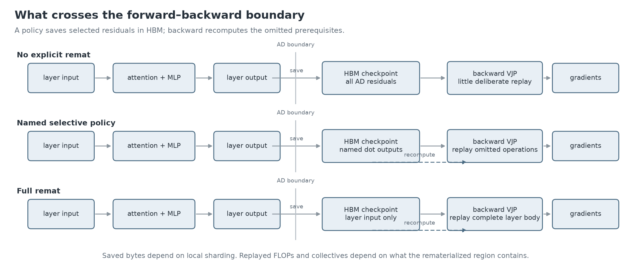
Rematerialization changes the storage-versus-recomputation tradeoff.

Instead of retaining every residual required by the backward pass, the system chooses selected checkpoint boundaries and reconstructs missing values when they are needed later. The method was developed for deep networks by Chen et al.; the JAX Scaling Book derivation relates the same trade to Transformer layers.

Let (\mathcal C(p)) be operations replayed under policy (p), and let (m_i) be the number of replays of operation (i). Then

\[F_{\mathrm{executed}}(p) =F_{\mathrm{ordinary\ step}} +\sum_{i\in\mathcal C(p)}m_iF_i.\]

Only operations inside the rematerialized region contribute replayed work. A policy that saves dot outputs may replay only normalization and pointwise work. Full layer remat can replay the projections and attention forward path.

The same rule applies to communication. A collective outside the checkpointed region executes once. A collective inside the region may be replayed during reconstruction.

The policy controls what crosses the autodiff boundary. Sharding changes the bytes represented by each checkpoint; the operations inside the rematerialized region determine replayed FLOPs and communication.

Implementing in JAX

jax.checkpoint and jax.remat are aliases. At a high level, a checkpoint policy answers a simple question for each operation:

May this value be saved, or must it be recomputed later?

Policies receive type-level primitive descriptions. Named policies use checkpoint_name, which is an identity at execution time and a label in the trace:

from jax.ad_checkpoint import checkpoint_name

def decoder_layer(x, weights):
    q = checkpoint_name(project_q(x, weights.q), "query_proj")
    context = checkpoint_name(attend(q, weights), "context")
    mlp = checkpoint_name(project_up(x, weights.up), "mlpwi_0")
    return combine(context, mlp)

policy = jax.checkpoint_policies.save_only_these_names(
    "query_proj", "context", "mlpwi_0"
)
checkpointed_layer = jax.checkpoint(decoder_layer, policy=policy)

The main policy constructors are:

Policy	Saved residuals
everything_saveable	Every residual that ordinary AD elects to keep
nothing_saveable or policy=None inside jax.checkpoint	Inputs to the remat boundary; internal values replay
dots_saveable and related dot policies	Dot outputs that satisfy the policy predicate
save_only_these_names(...)	Values carrying one of the listed names
save_and_offload_only_these_names(...)	Listed values kept on device or moved to another memory space

A common source of confusion is that policy=None does not disable rematerialization once a function has already been wrapped in jax.checkpoint. To disable explicit remat, call the original function. This distinction matters in framework dispatch code, where a config value first decides whether to wrap a layer and then selects the policy passed to that wrapper.

Use jax.ad_checkpoint.print_saved_residuals on a small shape before compiling the full model. It shows the AD decision before XLA fusion and buffer assignment. The optimized HLO and compiled.memory_analysis() are still required for the device-memory result.

MaxText policy surface

MaxText sets checkpoint_name on projections and context, resolves remat_policy, and applies the resulting policy to the decoder layer. The current definitions are in Decoder.get_remat_policy and the equivalent NNX policy builder. The NNX decoder explicitly calls the pure layer when remat_policy == "none".

MaxText value	Named values retained by the preset
minimal_with_context	Q/K/V or fused QKV, output projection, context, MLP up and down projections
minimal	The same projection classes without context
save_dot_with_context_except_mlp	Attention projections, output projection, and context
save_qkv_proj	Q/K/V or fused QKV projections
full	No internal values allowed by the default checkpoint policy
custom	Per-name device, remat, or offload assignments

The policy names are only meaningful if they match the names actually produced by the model implementation. MaxText’s minimal_with_context list contains names for separate Q/K/V, fused QKV, and gated MLP variants for this reason. A low-precision backend can add packed weights, scales, or quantization history that a BF16 policy never considered.

Changes at the HLO level

The following figure uses a real two-layer BF16 fixture. Without explicit remat, %tanh.3 feeds the backward %sub.3 directly. Full remat carries %remat2.10 through %remat2.11, then reconstructs the missing value with %dot_general.9 and %tanh.6; both carry checkpoint/rematted_computation in their literal metadata.

Real JAX 0.11 `before_optimizations` HLO rendered with Graphviz. Exact operation names and shapes are retained; layout-only and unrelated gradient nodes are pruned.

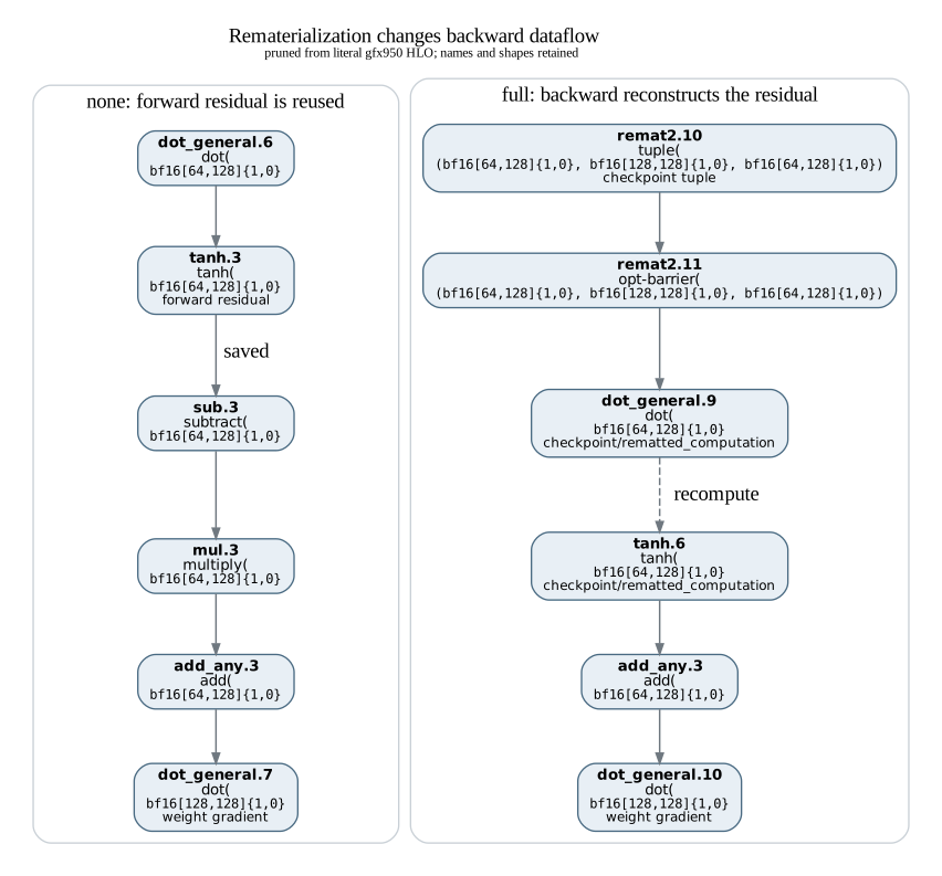
The appearance of additional HLO operations does not, by itself, prove that memory has been reduced. The useful checks are a smaller forward-to-backward residual tuple, reconstructed work in the backward body, and a shorter peak live range in the buffer assignment. XLA’s own compiler rematerialization may also replay operations for scheduling reasons; that is separate from the explicit JAX policy.

Sharding and collectives

Sharding affects checkpoint size only when it reduces the local shape of a saved tensor. If a global activation is ([B,S,D]) and its batch and hidden axes are sharded by (p_B) and (p_D), its local storage is

\[M_{\mathrm{local}}=\frac{BSDw}{p_Bp_D}.\]

Replicated sequence or hidden dimensions contribute no divisor. The Llama comparison below keeps four sequences per GPU while increasing global batch from 4 to 32 under FSDP-8, so its local named-activation estimate remains 45.5 GiB. FSDP greatly reduces the local parameter and optimizer state, but weak scaling does not reduce the local batch activations.

A collective is replayed only when it lies inside the rematerialized computation. For example, an FSDP weight AllGather performed before a checkpoint boundary can feed both forward and backward without being rematerialized. A gather inside a checkpointed layer can execute again when that layer is reconstructed.

The retained FSDP-8 scheduled HLO makes that distinction visible. All three policies contain eight static collective-start instructions and 1.076 GiB of summed result shapes. minimal_with_context and full each place one AllGather under checkpoint/rematted_computation; none places none there. The identical static counts do not prove that additional communication occurred at runtime. They show that the remat boundary contains a collective in this implementation, so dynamic execution must be counted from the loop structure or a device trace.

Case study: Llama 7B

The matched model has 6.738 billion parameters, 32 scanned layers, width 4096, MLP width 11008, 32 heads of width 128, sequence 4096, and local batch 4. Compute is BF16; parameters, gradients, and Adam moments are FP32. Transformer Engine attention is pinned to the CK/AITER route. Every run uses 30 synchronized steps on MI355X, and the table reports steps 10–29. The memory logger divides by (2^{30}), so its historical GB field is GiB.

The one-GPU cohort was captured on 16 September 2026 with JAX 0.11.0, ROCm plugin/PJRT 0.11.0.post1, ROCm 7.14, and local Llama source commit 5f996a88. The FSDP-8 cohort was captured on 11 September with JAX 0.11.0 and ROCm 7.14 using the same raw-JAX model and an eight-device fsdp mesh.

Scope	Policy	Median step	Std. dev.	Tokens/s/GPU	Compiled memory	Allocator peak
1 GPU	none	0.745 s	0.0010 s	21,992	247.6 GiB	247.56 GiB
1 GPU	minimal_with_context	0.676 s	0.0013 s	24,237	152.9 GiB	152.88 GiB
1 GPU	full	0.794 s	0.0020 s	20,635	106.6 GiB	106.62 GiB
FSDP-8	none	0.763 s	0.0006 s	21,473	150.5 GiB	150.49 GiB
FSDP-8	minimal_with_context	0.740 s	0.0020 s	22,141	66.9 GiB	66.86 GiB
FSDP-8	full	0.864 s	0.0037 s	18,963	21.1 GiB	21.14 GiB

Among the evaluated policies, minimal_with_context provides the best tradeoff between memory consumption and throughput. It is faster than none while using much less memory. On one GPU it removes 94.7 GiB from the compiled plan and improves median step time by 9.3%. Under FSDP-8 it removes 83.6 GiB and improves time by 3.0%. The results illustrate that retaining more activations is not automatically faster. Additional saved state increases memory traffic and can restrict scheduling flexibility.

The predicted 45.5 GiB named-residual term can be checked directly. Moving from minimal_with_context to full removes 46.3 GiB on one GPU and 45.8 GiB under FSDP-8. The close match validates the scale of the estimate; the remaining fraction belongs to alignment and other changed live ranges.

For full remat, the large decoder operations replayed in one forward layer stack are approximately

\[F_{\mathrm{replay,full}} =212.21\ \text{TFLOP}_{\mathrm{projections}} +17.59\ \text{TFLOP}_{\mathrm{attention}} =229.80\ \text{TFLOP}.\]

That is 32.7% of the ordinary 702.28-TFLOP model ledger, before pointwise work. Measured median time rises by 17.5% from minimal to full on one GPU and 16.8% under FSDP-8. A separate one-layer PMC capture confirms the direction: the profiler’s BF16 MFMA operation count is 35.031 TFLOP for none, 35.340 for minimal, and 38.072 for full. The one-layer step includes the vocabulary head, so its 8.7% full-versus-none counter increase is not the 32-layer analytical ratio.

The FSDP rows are weak scaling: local tokens stay at 16,384 while global batch grows to 32 sequences. They show that the remat choice must be retested after sharding. The smaller state leaves far more HBM headroom, while AllGather and ReduceScatter raise the cost of the full policy.

Attention backend implementations

Components of attention

Attention combines three tensors: queries, keys, and values. The forward pass computes attention scores, normalizes them with softmax, and uses the resulting probabilities to mix the value vectors.

\[S=\frac{QK^\mathsf T}{\sqrt d}+M,\qquad P=\operatorname{softmax}(S),\qquad O=PV,\]

where (M) contains the causal or padding mask. Backward has two matrix paths:

\[\begin{aligned} dV &= P^\mathsf T dO, & dP &= dO\,V^\mathsf T,\\ dS &= P\odot\left(dP-\operatorname{rowsum}(dP\odot P)\right),\\ dQ &= dS\,K, & dK &= dS^\mathsf TQ. \end{aligned}\]

A backend must implement the requested mask, layout, dtype, dropout, and sharding in both directions. A fast forward kernel with no correct VJP is an inference path. The backward equations also show why a training backend needs Q, K, V, and softmax information even when the forward API returns only O.

Forward and backward working sets

The key systems difference between standard attention and FlashAttention is memory.

A conventional implementation materializes score-like tensors whose size scales with both query length and key length. If (c) score or probability arrays are live, its HBM term is approximately

\[M_{\mathrm{standard}} \approx c\,B_\ell H_\ell S_qS_k w_s.\]

For the Llama shape ([B,H,S,S]=[4,32,4096,4096]), one FP32 score tensor is 8 GiB. The XLA path can have masked logits, exponentials, and normalized probabilities with overlapping lifetimes.

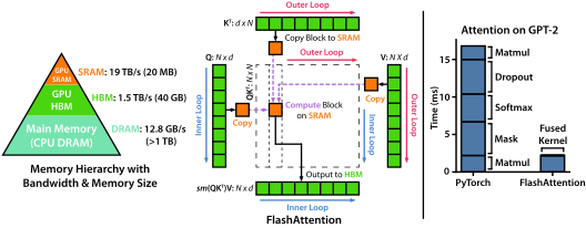
FlashAttention tiles Q, K, and V, maintains an online softmax, and avoids writing the complete (S_qS_k) matrix to HBM. A simple on-chip working-set model for one tile is

\[M_{\mathrm{tile}} \approx w\left[(B_q+2B_k)d+B_qB_k+B_qd_v\right],\]

plus (O(BHS)) row statistics in HBM. The exact tile, staging depth, and accumulator layout are backend decisions. FlashAttention-2 also changes work partitioning to improve occupancy and parallelism.

Figure 1 from FlashAttention. The left panel shows the relevant mechanism: Q, K, and V tiles move through on-chip SRAM without materializing the full attention matrix in HBM. The right panel is the paper's A100 result and is not an MI355X measurement.

Backward attention should be considered a separate implementation problem rather than a consequence of forward performance. It may reconstruct scores from Q, K, the output, and row log-sum-exp; calculate (dQ) separately from (dK,dV); use atomics; and launch conversion or reduction helpers. Forward timing or a forward-only HLO fixture cannot predict those costs.

ROCm attention backends

From the user’s perspective, MaxText exposes several attention implementations that produce the same mathematical result through different execution paths. The corresponding standard, TE, and Pallas selection is in AttentionOp.apply_attention.

Route	Forward implementation	Backward ownership	What HLO reveals
Standard XLA	QK dot, mask, reductions, exponential, normalization, PV dot	JAX transposes the exposed primitives; XLA selects kernels for the resulting graph	Algorithm and tensors remain visible
Transformer Engine	DotProductAttention, selected in MaxText by attention=cudnn_flash_te	TE custom VJP and te_fused_attn_backward_ffi	Typed FFI boundary, outputs, layouts, attributes, and workspace contract
Direct JAX-AITER	jax_aiter.mha.flash_attn_func	JAX-AITER custom VJP; unified forward and backward FFI handlers	MhaFwdUnifiedJA and MhaBwdUnifiedJA boundaries
Tokamax Pallas–Triton	Pallas flash-attention program compiled through Triton	Pallas forward-residual and VJP kernels	Generated fusions and kernel metadata rather than an external library call

cudnn_flash_te is a compatibility name in MaxText; it enters Transformer Engine’s JAX module. On ROCm, TE filters the problem by dtype, shape, QKV layout, mask, dropout, and head dimensions, then selects an enabled backend. The ROCm Transformer Engine source documents CK and AOTriton, with CK taking priority when both match. The experiment sets NVTE_FUSED_ATTN_CK=1 and NVTE_FUSED_ATTN_AOTRITON=0.

Direct JAX-AITER bypasses Transformer Engine’s backend selection layer and invokes the JAX-AITER implementation directly. The pinned source at 35b7175c registers one FFI target per direction and supplies custom partitioning plus a custom VJP. AITER still chooses CK or ASM internally from the concrete problem.

The Pallas route is the only one whose flash algorithm is expressed as a JAX kernel program. Current MaxText uses attention=flash on GPU to construct PallasTritonFlashAttention. The Llama experiment pins Tokamax 0.0.14, supplies an explicit BF16 dot algorithm, and adjusts Tokamax’s GPU capability guard for gfx950. Its result therefore belongs to that wrapper and version, not to every Pallas/Triton configuration.

Changes at the HLO level

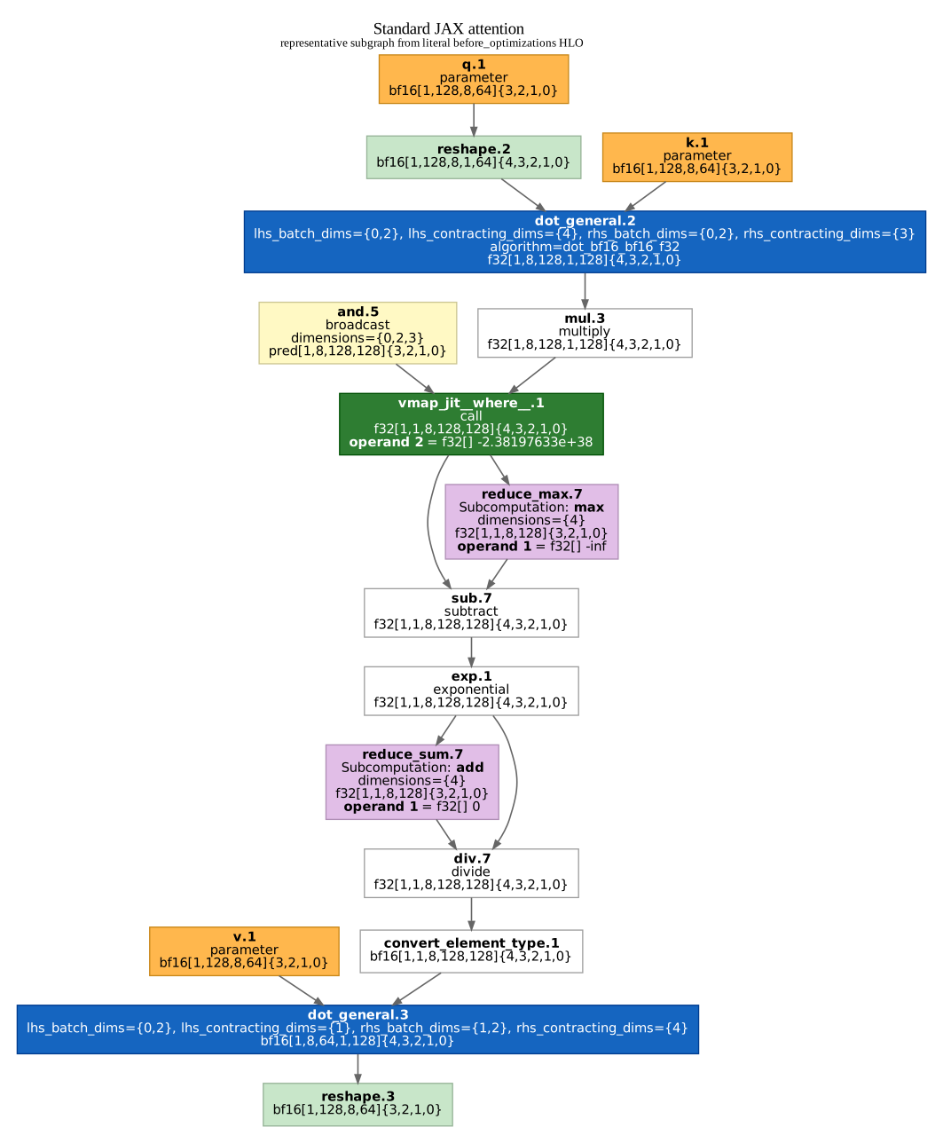
In standard attention, the compiler can see the score computation, masking operations, softmax reductions, and value-mixing output explicitly.

The matched forward fixtures use BF16 Q, K, and V shaped [1,128,8,64]. Their HLO contains %dot_general.2, the causal selection, FP32 %reduce_max.7, %exp.1, %reduce_sum.7, %div.7, and the final %dot_general.3.

Real JAX 0.11 `before_optimizations` HLO. The score path is visible as ordinary HLO and uses FP32 for the softmax-shaped tensors.

Transformer Engine instead produces custom_call_target="te_fused_attn_forward_ffi". Its tuple contains the BF16 output, FP32 row state, RNG state, and a byte result before %te_fused_attn_forward_ffi.6 extracts the output.

Real JAX 0.11 `before_optimizations` HLO. The graph shows the TE typed-FFI boundary and its result contract; kernel internals remain outside HLO.

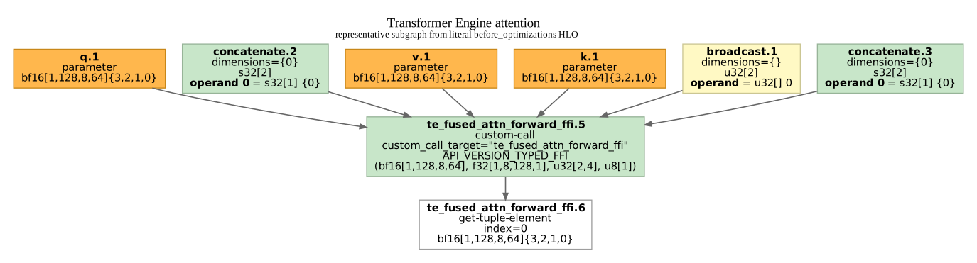
These graphs describe only the forward computation visible to HLO. The TE source defines the separate te_fused_attn_backward_ffi; the full training trace below establishes the kernels selected behind both directions. This is the OpenXLA custom-call boundary: HLO describes the external operation, while the host handler enqueues work on the ROCm stream.

Observed kernel geometry

The one-layer capture uses the production attention shape: BF16, batch 4, sequence 4096, 32 heads, and head dimension 128. The trace records grid, workgroup, LDS, regular VGPR, and accumulator VGPR fields. It does not report a universal attention tile, so the figure preserves those fields rather than inferring (B_q) and (B_k).

Observed launch geometry from the 10 September one-layer PMC campaign. Transformer Engine and direct JAX-AITER reach the same named forward kernel and geometry, then use different backward kernels. The fields are literal CSV values.

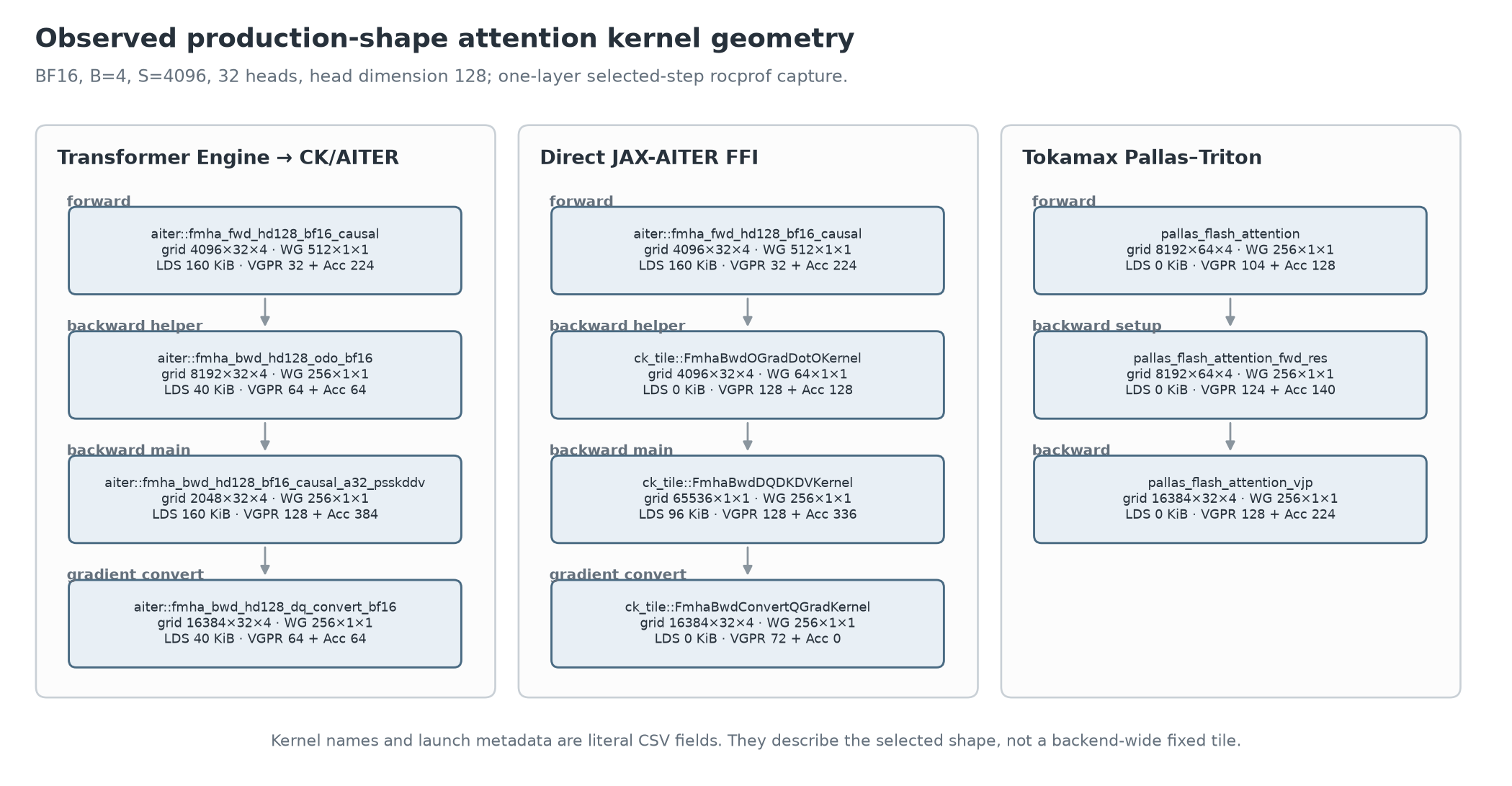
Both TE and direct JAX-AITER launch aiter::fmha_fwd_hd128_bf16_causal with grid 4096×32×4, a 512-thread workgroup, 160 KiB LDS, 32 VGPRs, and 224 accumulator VGPRs. At this shape, the observed forward kernel is identical across the Transformer Engine and direct JAX-AITER paths.

The forward kernels converge, but the backward implementations diverge. TE launches the named AITER O-gradient helper, ...bf16_causal_a32_psskddv, and dQ conversion kernels. Direct JAX-AITER launches CK Tile classes including FmhaBwdOGradDotOKernel, FmhaBwdDQDKDVKernel, and FmhaBwdConvertQGradKernel. Pallas launches pallas_flash_attention_fwd_res and pallas_flash_attention_vjp. The resource fields show substantial register and LDS pressure, but this campaign did not collect the level counters needed to calculate achieved occupancy. Chapter 1’s occupancy formula should not be applied to these fields as though it were a measured value.

Case study: Llama 7B

The retained clean timing comparison comes from docker.io/rocm/jax-training:maxtext-v26.5 with JAX 0.10.0 on one MI355X. Both rows use the raw-JAX Llama model, BF16, sequence 4096, batch 4, minimal_with_context, 30 synchronized steps, and the same XLA flags. The table uses steps 10–29.

Attention route	Median step	Tokens/s/GPU	Compiled memory	Allocator peak
Standard XLA	1.498 s	10,934	167.1 GiB	167.07 GiB
Transformer Engine CK/AITER	0.662 s	24,758	152.1 GiB	152.09 GiB

For this complete training step, Transformer Engine delivers both higher throughput and lower peak memory usage. Median step time falls from 1.498 s to 0.662 s, a 2.26× speedup, while peak memory falls by 15.0 GiB.

The magnitude of the speedup exceeds attention’s share of model FLOPs because FLOP counts alone do not describe execution time. They omit score traffic, softmax work, launches, and backend efficiency.

The 10 September JAX 0.11 PMC campaign ran one production-shaped layer and selected one warmed training step. Each counter group ran in a fresh process. The totals below cover the complete one-layer step, not only the attention kernels.

Route	BF16 MFMA operations	HBM fetch	HBM write	L2 hit rate
Standard XLA	36.377 TFLOP	135.354 GiB	49.304 GiB	61.68%
Transformer Engine	35.179 TFLOP	79.426 GiB	19.966 GiB	69.59%
Direct JAX-AITER	35.147 TFLOP	81.047 GiB	20.825 GiB	69.77%
Pallas–Triton	37.742 TFLOP	96.315 GiB	17.641 GiB	68.46%

The installed gfx950 counter definitions give the formulas:

\[\begin{aligned} F_{\mathrm{MFMA,BF16}} &=512\sum \texttt{SQ\_INSTS\_VALU\_MFMA\_MOPS\_BF16},\\ R_{\mathrm{HBM}}[\mathrm{GiB}] &=\frac{\sum\texttt{FETCH\_SIZE}[\mathrm{KiB}]}{2^{20}},\\ W_{\mathrm{HBM}}[\mathrm{GiB}] &=\frac{\sum\texttt{WRITE\_SIZE}[\mathrm{KiB}]}{2^{20}},\\ h_{\mathrm{L2}} &=\frac{\sum\texttt{TCC\_HIT\_sum}} {\sum(\texttt{TCC\_HIT\_sum}+\texttt{TCC\_MISS\_sum})}. \end{aligned}\]

The ROCprofiler-SDK counter service serializes dispatches for per-kernel counting. PMC timestamps and step duration are therefore excluded from the speed table. The counters support the mechanism: all three flash-style routes move much less HBM data than standard XLA in this matched one-layer step. They do not supply a clean four-way runtime ranking.

Grouped GEMM kernels for MoE

Why MoE requires grouped GEMM

Mixture-of-Experts introduces a challenge that does not exist in dense models: each expert receives a different number of tokens.

Let (T) be the number of input tokens and (k) the number of experts selected per token. If expert (e) receives (n_e) rows,

\[\sum_{e=1}^{E}n_e=Tk, \qquad \bar n=\frac{Tk}{E}.\]

The (n_e) values depend on data and router parameters. Because the expert workloads are uneven, a single dense batch shape cannot represent the routed computation efficiently. Four implementation choices are useful:

1. Dense masked evaluates all (E) experts for every token and later selects the routed outputs. It performs (E/k) times the ideal routed expert arithmetic.
2. Fixed capacity allocates (C) rows per expert, pads underfull experts, and drops assignments beyond (C).
3. A ragged operation keeps the (n_e) values but can lower to a masked, dense-padded batch.
4. Grouped GEMM submits one runtime (M=n_e) problem per expert to one grouped library operation.

An illustrative routed layer. Dense masked runs every expert, fixed capacity reserves equal slots, and a dense-padded ragged lowering masks padded rows. Grouped GEMM retains one runtime row count per expert; hardware tile tails still remain.

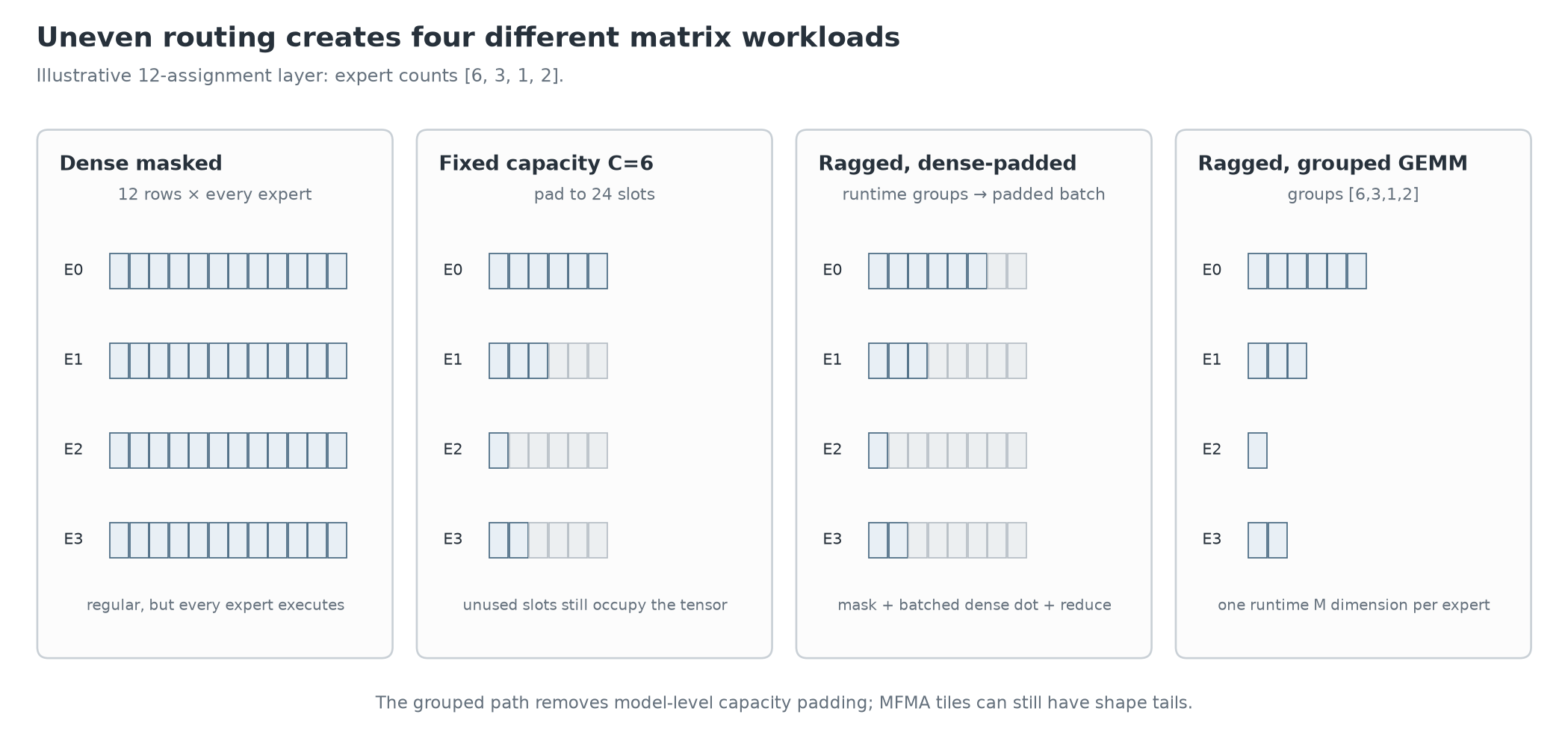
For a row tile (T_M), a padded-work upper model is

\[\tilde n_e=\left\lceil\frac{n_e}{T_M}\right\rceil T_M, \qquad W_{\mathrm{pad}} =\frac{\sum_e\tilde n_e-\sum_en_e}{\sum_en_e},\]

and an expert GEMM with contracting width (K) and output width (N) issues

\[F_{\mathrm{padded}}=2KN\sum_e\tilde n_e \quad\text{instead of}\quad F_{\mathrm{useful}}=2KN\sum_en_e.\]

Predication can avoid some arithmetic, so this is an upper model of row-tile waste. It still captures the utilization loss from small or empty groups. Grouped GEMM removes fixed-capacity padding from its API contract; it cannot remove MFMA shape tails or create enough rows for an underloaded expert.

Router to expert and back

Conceptually, sparse MoE execution consists of four stages:

route → move tokens → run expert GEMMs → combine outputs.

MaxText expands these stages into five steps:

1. The router produces top-k expert indices and weights.
2. MaxText repeats each token k times, sorts by destination expert, and calculates group_sizes.
3. A ragged AllToAll sends rows to the expert owners, which sort them by local expert.
4. Grouped up, gate, and down GEMMs process the routed rows.
5. MaxText reverses the local sort and AllToAll, restores token order, and combines each token’s k outputs with the router weights.

The current RoutedMoE.sparse_matmul constructs the local GMM function. Routing repeats and sorts assignments, then obtains group sizes with jnp.bincount. With expert parallelism, the dispatch and return use jax.lax.ragged_all_to_all.

The handoff inside the layer is concise:

x, routing, route_metadata = route(x, logits, pre_bias_logits, rngs)
gmm_fn = get_gmm_for_local_experts(x, routing, route_metadata)
output0, output1 = gmm_up(x, w0, w1, w0_bias, w1_bias, gmm_fn, weight_gather)
intermediate = apply_ffn_activation(output0, output1)
expert_output = gmm_fn(intermediate, wo, tiling=wo_tile_size, ...)
output = unpermute(expert_output, routing.sorted_selected_experts, routing.weights, ...)

This comes from the current route–GMM–combine body. The sparse algorithm includes sorting and communication around the expert matrix products. A grouped GEMM microbenchmark excludes most of the layer cost.

MaxText controls

The current user-facing MaxText field is sparse_matmul. A noteworthy implementation detail is that current MaxText does not expose a user-facing use_ragged_dot option.

MaxText fields	JAX-level expert path
sparse_matmul=false, capacity_factor<0	Dense masked expert contractions
sparse_matmul=false, capacity_factor>0	Fixed-capacity dispatch, expert, and combine contractions
sparse_matmul=true, use_tokamax_gmm=true	Tokamax ragged-dot implementation
sparse_matmul=true, use_tokamax_gmm=false, megablox=true	MaxText’s older Megablox path
sparse_matmul=true, use_tokamax_gmm=false, megablox=false	jax.lax.ragged_dot

The dispatch is visible at RoutedMoE.__call__. The legacy config validator also sets the internal JAX option jax_ragged_dot_use_ragged_dot_instruction for the last combination. That option is not a replacement user field.

The Mixtral launchers under test use:

sparse_matmul: true
megablox: false
use_tokamax_gmm: false
capacity_factor: -1.0
ragged_buffer_factor: -1.0
use_custom_sort_vjp: true

ragged_buffer_factor=-1.0 allocates MaxText’s worst-case receive buffer. It avoids buffer-induced assignment drops, but unused buffer rows still consume memory. use_custom_sort_vjp=true makes the sort backward apply the inverse permutation instead of relying on a generic gather gradient.

Grouped GEMM lowering paths

A common misconception is that jax.lax.ragged_dot automatically implies grouped GEMM execution.

It does not.

ragged_dot specifies the operation semantics. The backend remains free to lower those semantics either to dense padded computation or to a true grouped GEMM implementation. On this ROCm XLA build, the experiment separates two lowerings:

# Dense-padded lowering
XLA_FLAGS="--xla_gpu_enable_cublaslt=true \
  --xla_gpu_experimental_use_ragged_dot_grouped_gemm=false"

# hipBLASLt GroupedGEMM lowering
XLA_FLAGS="--xla_gpu_enable_cublaslt=true \
  --xla_gpu_experimental_use_ragged_dot_grouped_gemm=true"

The cublaslt spelling is shared GPU-backend compatibility vocabulary. OpenXLA’s GEMM rewriter selects hipBLASLt GroupedMatmul on ROCm, and its ROCm BLASLt runtime builds the grouped plan. hipBLASLt documents the underlying hipblaslt_ext::GroupedGemm API, including per-problem (m,n,k), algorithm selection, user arguments, and workspace.

This is an XLA library custom call, not XLA FFI. Transformer Engine now contains JAX MoE code, but the MaxText path and flags above do not select it. No TE or direct JAX-AITER training FFI appears in these four expert fixtures. A package being installed does not change the lowering without a frontend call and a matching custom-call target.

Changes at the HLO level

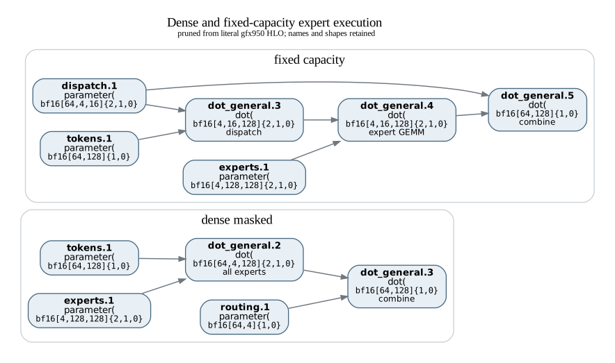
The first two real fixtures use 64 BF16 token rows, four experts, width 128, and capacity 16. Dense masked HLO forms %dot_general.2 with output bf16[64,4,128], so every token has an output for every expert. Fixed capacity first dispatches to bf16[4,16,128], applies the expert %dot_general.4, then combines with %dot_general.5.

Real JAX 0.11 `before_optimizations` HLO. Dense masked carries an expert dimension for every token. Fixed capacity carries an expert and capacity dimension through dispatch, expert GEMM, and combine.

The ragged pair begins with the same FP16 jax.lax.ragged_dot over 64 rows and four groups. With grouped lowering disabled, optimized HLO expands and masks rows in %loop_transpose_fusion, computes %gemm_fusion_dot.2 as f32[8,64,128], and reduces groups with %loop_reduce_fusion.

With grouped lowering enabled, the graph becomes one custom_call_target="__cublas$lt$groupedMatmul" consuming tokens, expert weights, and s32[4] group sizes. The result tuple contains f16[64,128] plus a 784-byte workspace.

Real JAX 0.11 gfx950 optimized HLO. The frontend operation is the same; the XLA flag changes its backend lowering. Exact operation names and shapes are retained.

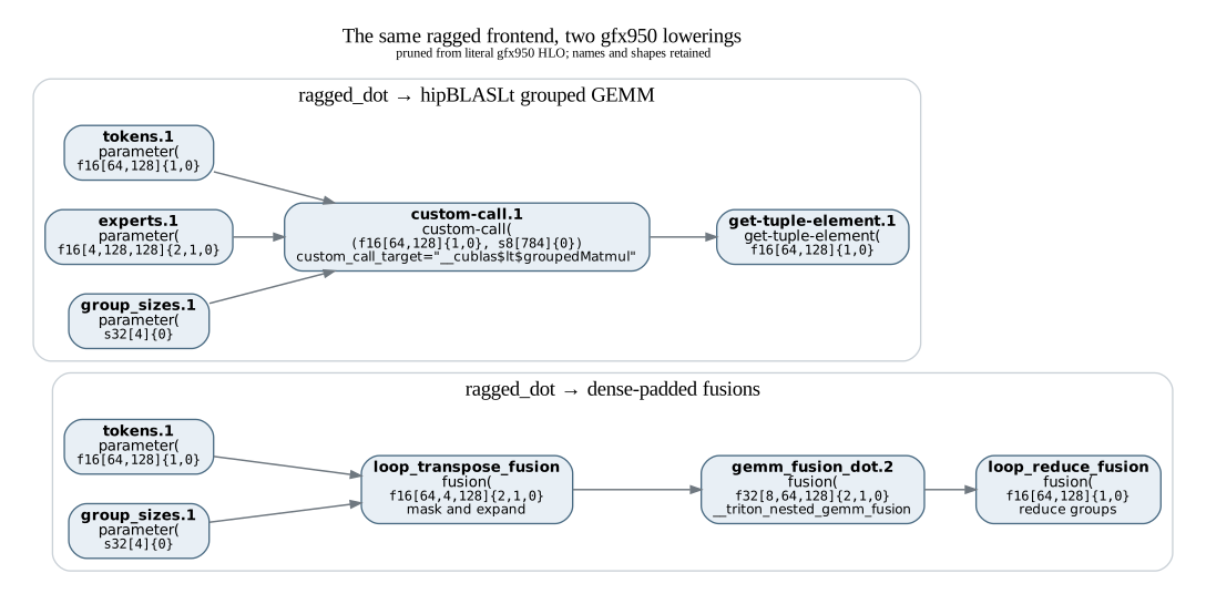
These fixtures isolate expert execution. They do not include the full Mixtral router, ragged AllToAll, three expert projections, rematerialization, or backward. For a model run, verify all of those in the optimized training HLO and identify the final library kernel in a device trace.

Case study: Mixtral 8x22B

The study model has 56 layers, width 6144, expert width 16384, eight experts, and top-2 routing. Sequence length is 4096, local batch is 4, and two gradient accumulation microsteps produce 262,144 input tokens per eight-GPU update. The current recipe uses Transformer Engine attention, scanned layers, and remat_policy=save_dot_with_context_except_mlp.

These measurements should be interpreted as integration checkpoints rather than controlled kernel comparisons. The rows come from separate captures, so the step times are not a comparison of the two meshes:

Mesh and expert path	Measured step	Tokens/s/GPU	Compiled memory
FSDP-1 / EP-8, BF16 fixed capacity	8.354 s	3,922.4	220.0 GiB/GPU
FSDP-4 / EP-2, BF16 fixed capacity	20.599 s	1,590.7	not recorded

Both rows show that the 140.63-billion-parameter model and fixed-capacity mesh can complete an update on eight MI355X GPUs. They do not compare ragged dense-padded with GroupedGEMM. The current v26.6 scripts define that matched FP16 pair with identical router, EP-8 mesh, worst-case ragged buffer, and AllToAll flags; only --xla_gpu_experimental_use_ragged_dot_grouped_gemm changes. Full 30-step timing, router histograms, drop counts, optimized full-model HLO, grouped-kernel traces, and exposed collective time remain the current integration work.

Applying the configuration sequence

The central lesson of the book is that optimization decisions are hierarchical.

precision → sharding → memory policy → kernel selection.

1. Choose the numeric recipe and optimizer-state dtypes.
2. Choose a mesh that makes persistent state fit and record each GPU’s local (B,S,D,F) shapes.
3. Estimate saved activations at those local shapes, then measure none, one named policy, and full. Keep collectives outside remat boundaries when the program permits it.
4. Select attention with separate forward and backward verification. Use HLO for the compiler boundary, a kernel trace for the implementation, and clean timing for the result.
5. For MoE, decide dropping and padding semantics before choosing a kernel. After ragged_dot, verify whether optimized HLO contains dense-padded work or the hipBLASLt grouped call.
6. Run PMCs only after a trace identifies the question. Counter collection explains MFMA and memory traffic; its serialized duration is not training throughput.

For the measured Llama shape, the remat sweep selects minimal_with_context, and the retained clean attention subset favors TE/CK-AITER over standard XLA while preserving substantial HBM headroom. Mixtral has reached the fixed-capacity stage; the matched ragged lowering and routing diagnostics are the remaining step before grouped GEMM can be selected.