Training in Mixed Precision
Chapter 4 of How to Scale Your Model on AMD (Chapter 3: Profiling a Training Step | Chapter 5: Sharding and Parallelism)
How BF16, FP16, FP8, and OCP microscaling recipes change JAX programs, MI355X matrix execution, memory use, and Llama 2 70B throughput.
Lower precision changes both the matrix instructions executed by the GPU and the amount of data moved through memory. It does not mean running an entire training step in FP8 or MXFP4.
Instead, modern training recipes keep long-lived state and numerically sensitive operations in wider formats, while converting selected operands to lower precision immediately before large matrix multiplications.
This chapter separates three kinds of number:
- Theoretical peak comes from the MI355X specification.
- Model prediction applies explicit assumptions to those peaks.
- Measurement comes from timed MaxText steps on eight MI355X GPUs.
Why train in lower precision
MI355X has separate dense matrix rates for its native input formats. At the published 2.4 GHz peak clock, the format ceiling is
\[C_{\mathrm{format}} =256\ \mathrm{CUs} \times F_{\mathrm{format}} \frac{\mathrm{FLOPs}}{\mathrm{clock\cdot CU}} \times 2.4\times10^9\ \frac{\mathrm{clocks}}{\mathrm{s}}.\]The MI355X product brief gives $F_{\mathrm{format}}=4096$ for BF16/FP16, $8192$ for OCP FP8/MXFP8, and $16384$ for MXFP6/MXFP4. The corresponding dense, non-sparse peaks are:
| Matrix operands | Dense theoretical peak per GPU | Ratio to BF16 |
|---|---|---|
| BF16 or FP16 | 2.5166 PFLOP/s | 1× |
| OCP FP8 or MXFP8 | 5.0332 PFLOP/s | 2× |
| MXFP6 or MXFP4 | 10.0663 PFLOP/s | 4× |
These numbers describe peak matrix throughput, not end-to-end training speed. Converting an MLP projection to MXFP4 does not make softmax, normalization, communication, optimizer updates, or kernel-launch overhead four times faster. Only the portions of the training step that actually execute on lower-precision matrix hardware can benefit from the higher peak rate.
Higher matrix throughput is only half of the story. Lower-precision formats also reduce the amount of data stored in memory and moved through the memory hierarchy.
An unscaled tensor with $n$ elements at $b$ bits per element occupies
\[M_{\mathrm{tensor}}(n,b)=\frac{nb}{8}\ \mathrm{bytes}.\]A BF16 tensor therefore uses twice the payload of FP8 and four times the payload of packed FP4. Smaller operands take less HBM capacity and bandwidth, and a saved FP8 activation for Wgrad uses half the space of a BF16 copy. Scale arrays, padding, transposed representations, and workspaces add bytes; optimizer state may not shrink at all.
The original JAX Scaling Book roofline chapter connects this byte count to arithmetic intensity and the HBM bandwidth bound.
Higher precision still has defined jobs:
- FP32 master parameters preserve small optimizer updates.
- FP32 moments and selected gradients preserve optimizer state.
- FP32 partial sums reduce error across a long contraction.
- BF16 commonly carries layer inputs and outputs between low-precision GEMMs.
- FP32 remains useful for reductions, loss computation, logits, and normalization statistics.
The goal is to spend narrow formats where MI355X has faster matrix instructions or where saved bytes matter, while retaining wider formats for the roles that need them.
What mixed precision means
When people refer to an “FP8 model”, they are usually collapsing several separate datatype decisions into a single label.
In practice, a matrix multiplication involves at least four distinct precisions:
\[C_{\mathrm{stored}} =\operatorname{cast}_{t_{\mathrm{out}}} \left( \operatorname{accum}_{t_{\mathrm{acc}}} \left[ Q_{t_A}(A)\,Q_{t_B}(B) \right] \right).\]$t_A$ and $t_B$ describe the two encoded operands, $t_{\mathrm{acc}}$ the accumulator, and $t_{\mathrm{out}}$ the stored output. $Q$ also includes a scaling policy when the encoded format cannot cover the source tensor’s range. Forward propagation, activation-gradient GEMM (Dgrad), and weight-gradient GEMM (Wgrad) can make different choices.
CDNA 4 exposes this separation in its instruction set. For example,
v_mfma_scale_f32_16x16x128_f8f6f4 consumes scaled 8-, 6-, or 4-bit
operands and updates FP32 accumulators. The
CDNA 4 ISA
defines the operand and scale layouts. A kernel can then store a BF16 output.
Using that instruction for one projection says nothing about the dtype of
RMSNorm, softmax, the residual stream, or Adam.
AMD’s
CDNA 4 FP8 GEMM guide
shows how those instruction-scale fragments fit into a complete GEMM kernel.
This distinction also separates storage format from compute format.
A weight might be stored as an FP32 optimizer parameter, gathered by FSDP, cast to BF16, quantized to FP8 or MXFP4 for a single GEMM, and then discarded. Calling such a system an “FP8 model” hides most of the machinery that actually determines memory usage and numerical behavior.
DeepSeek-V3 FP8 recipe
DeepSeek-V3 provides a useful example of how these choices come together in a production training recipe. Its Section 3.3.1 defines the mixed-precision framework and Figure 6 shows one linear layer across forward and backward propagation.
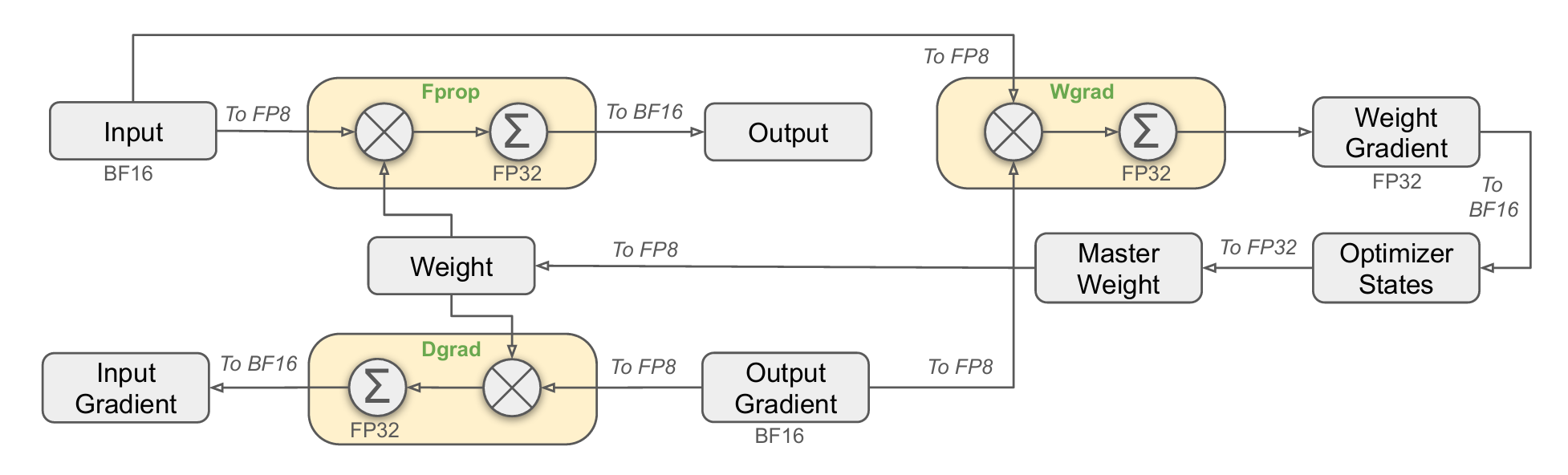
For the illustrated linear operator:
| GEMM | FP8 operands | Accumulation | Stored result |
|---|---|---|---|
| Fprop | layer input, weight | FP32 | BF16 layer output |
| Dgrad | output gradient, weight | FP32 | BF16 input gradient |
| Wgrad | saved layer input, output gradient | FP32 | FP32 weight gradient |
The report keeps embeddings, the output head, MoE gates, normalization, and attention in BF16 or FP32. Master weights and gradients remain FP32; its AdamW moments are BF16. This is what “mixed precision” means in practice. The highest-FLOP matrix multiplications use FP8 operands, while model state and numerically sensitive parts of the training loop remain in BF16 or FP32.
DeepSeek adds two controls around those GEMMs:
- Activations use one online scale per $1\times128$ tile, meaning one token row and 128 channels. Weights use one scale per $128\times128$ block. Smaller groups isolate feature outliers and let every operand use E4M3.
- On the H800 implementation, matrix partial sums are promoted to FP32 every $N_C=128$ positions along the contraction. The same point applies the per-group dequantization scales.
That accumulation procedure describes DeepSeek’s H800 kernels. On MI355X, the analogous design question is which CDNA 4 scaled MFMA form, FP32 accumulator, and scale layout the ROCm kernel uses. The common principle is high-precision accumulation of scaled low-precision products, not identical machine instructions.
DeepSeek also stores selected linear activations in FP8 for Wgrad and sends selected MoE activations in FP8, while retaining BF16 combine paths. Those choices target memory and network bytes independently of the model’s durable state.
Precision and quantization formats
The format selects a set of representable values. The recipe selects where the format is used, how tensors are scaled, what accumulates the dot product, and which representation is saved for backward.
| Format | Element encoding | Maximum finite magnitude | Scaling unit | Effective storage | MI355X dense peak |
|---|---|---|---|---|---|
| BF16 | S1 E8 M7 | $3.39\times10^{38}$ | none | 16 bits/value | 2.5166 PFLOP/s |
| FP16 | S1 E5 M10 | 65,504 | often loss scale | 16 bits/value | 2.5166 PFLOP/s |
| OCP FP8 E4M3 | S1 E4 M3 | 448 | commonly per tensor | 8 bits/value | 5.0332 PFLOP/s |
| OCP FP8 E5M2 | S1 E5 M2 | 57,344 | commonly per tensor | 8 bits/value | 5.0332 PFLOP/s |
| MXFP8 | E4M3 or E5M2 | scale-dependent | E8M0 per 32 | 8.25 bits/value | 5.0332 PFLOP/s |
| MXFP6 | E3M2 or E2M3 | scale-dependent | E8M0 per 32 | 6.25 bits/value | 10.0663 PFLOP/s |
| MXFP4 | E2M1 | scale-dependent | E8M0 per 32 | 4.25 bits/value | 10.0663 PFLOP/s |
The maximum-magnitude column is for an unscaled scalar encoding. MX range is the product of an element value and its block scale. Effective storage counts one eight-bit scale per full 32-element block and excludes padding and extra row/column representations.
BF16 and FP16
BF16 preserves FP32’s eight exponent bits and keeps seven explicit fraction bits. FP16 devotes ten bits to the fraction but only five to the exponent. BF16 therefore has FP32-like range with coarser spacing; FP16 has finer spacing near one and a much smaller range.
On MI355X, both formats typically accumulate into FP32 and share the same theoretical matrix peak. The practical differences are numerical range, representable values, and the specific kernels selected for a given workload. FP16 training commonly combines an FP32 master weight with loss scaling:
\[g_{16}=\operatorname{cast}_{16}(L g),\qquad g_{32}=\operatorname{cast}_{32}(g_{16})/L,\]where $L$ shifts small gradient values into FP16’s representable range before the optimizer update. The original mixed-precision training paper describes FP32 master weights, FP16 arithmetic, and loss scaling. BF16’s exponent range usually removes the need for that gradient shift.
OCP FP8
The OCP 8-bit Floating Point Specification standardizes two encodings:
- E4M3 uses four exponent and three fraction bits. It offers more precision.
- E5M2 uses five exponent and two fraction bits. It offers more range.
The usual hybrid recipe uses E4M3 for forward activations and weights and E5M2 for backward gradients. The FP8 Formats for Deep Learning paper introduced this division and evaluated it through 175-billion-parameter language models.
FP8’s reduced numerical range makes scaling a necessary part of the representation. Before conversion, tensors are scaled so that their values make effective use of the available FP8 range.
For a simple absmax per-tensor scale,
\[a=\max_i |x_i|,\qquad s=\frac{a}{q_{\max}},\qquad q_i=\operatorname{round}\!\left( \operatorname{clip}\left(\frac{x_i}{s},-q_{\max},q_{\max}\right) \right),\qquad \hat{x}_i=sq_i.\]Current scaling computes $a$ from the tensor being converted. Delayed scaling uses an amax history from earlier steps, avoiding a current-tensor reduction on the critical path. Transformer Engine’s delayed recipe stores a scale and amax history for each quantized tensor. Its current recipe computes the scale as the tensor flows through the operation.
The scale is therefore part of the tensor’s representation. An FP8 payload without its corresponding scale is incomplete because the original magnitude information has been lost.
MXFP8, MXFP6, and MXFP4
The OCP Microscaling Formats Specification defines blocks of $k=32$ elements sharing one E8M0 scale. E8M0 is an eight-bit exponent-only value, so each scale is a power of two. If each element uses $b$ bits and the shared scale uses $s$ bits, a full block costs
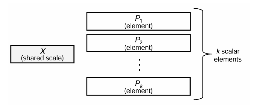
For $k=32$ and $s=8$, MXFP8, MXFP6, and MXFP4 use 8.25, 6.25, and 4.25 effective bits per element. A complete block occupies 33, 25, or 17 bytes respectively.
The element formats are:
- MXFP8: E4M3 or E5M2 elements;
- MXFP6: E3M2 or E2M3 elements;
- MXFP4: E2M1 elements.
Block scaling assigns a scale to a small group of values rather than an entire tensor. This makes it easier to accommodate local outliers and typically produces better numerical behavior than a single tensor-wide scale.
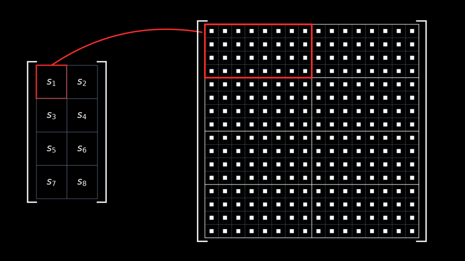
Rowwise and columnwise quantization are distinct because changing the block direction changes group membership. Training libraries often produce both representations from the wider source so Fprop, Dgrad, and Wgrad can consume the orientation they need.
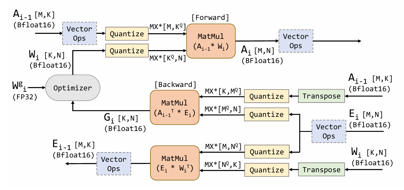
The OCP paper Microscaling Data Formats for Deep Learning uses this compute flow: dot-product operands are converted to MX, dot products return a scalar BF16/FP32 format, vector operations remain wider, and FP32 master weights receive the update.
Numerical controls and evidence
A low-precision training recipe should specify concrete controls:
- Scope. Select GEMM inputs rather than changing normalization, softmax, residual, loss, and optimizer tensors together.
- Range. Select E4M3 or E5M2 by tensor role, then choose per-tensor, per-tile, or 32-element block scales.
- Scale timing. Use current amax when the current distribution should set the scale, or a defined history for delayed scaling.
- Accumulation. Keep long dot products in FP32 and return wider outputs.
- State. Retain master weights and optimizer moments at the precision required by the optimizer.
- Rounding and orientation. Define round-to-nearest or stochastic rounding, and derive each rowwise or columnwise MX representation from the wider source.
The FP8 paper matched 16-bit training quality across CNN, RNN, and Transformer workloads up to 175B parameters. DeepSeek-V3 applied its fine-grained FP8 framework during a 14.8-trillion-token pretraining run. The MX paper demonstrated generative language-model training with sub-8-bit weights, activations, and gradients using its reported MX recipes. A new model and optimizer still need their own quality gate.
Implementing in JAX
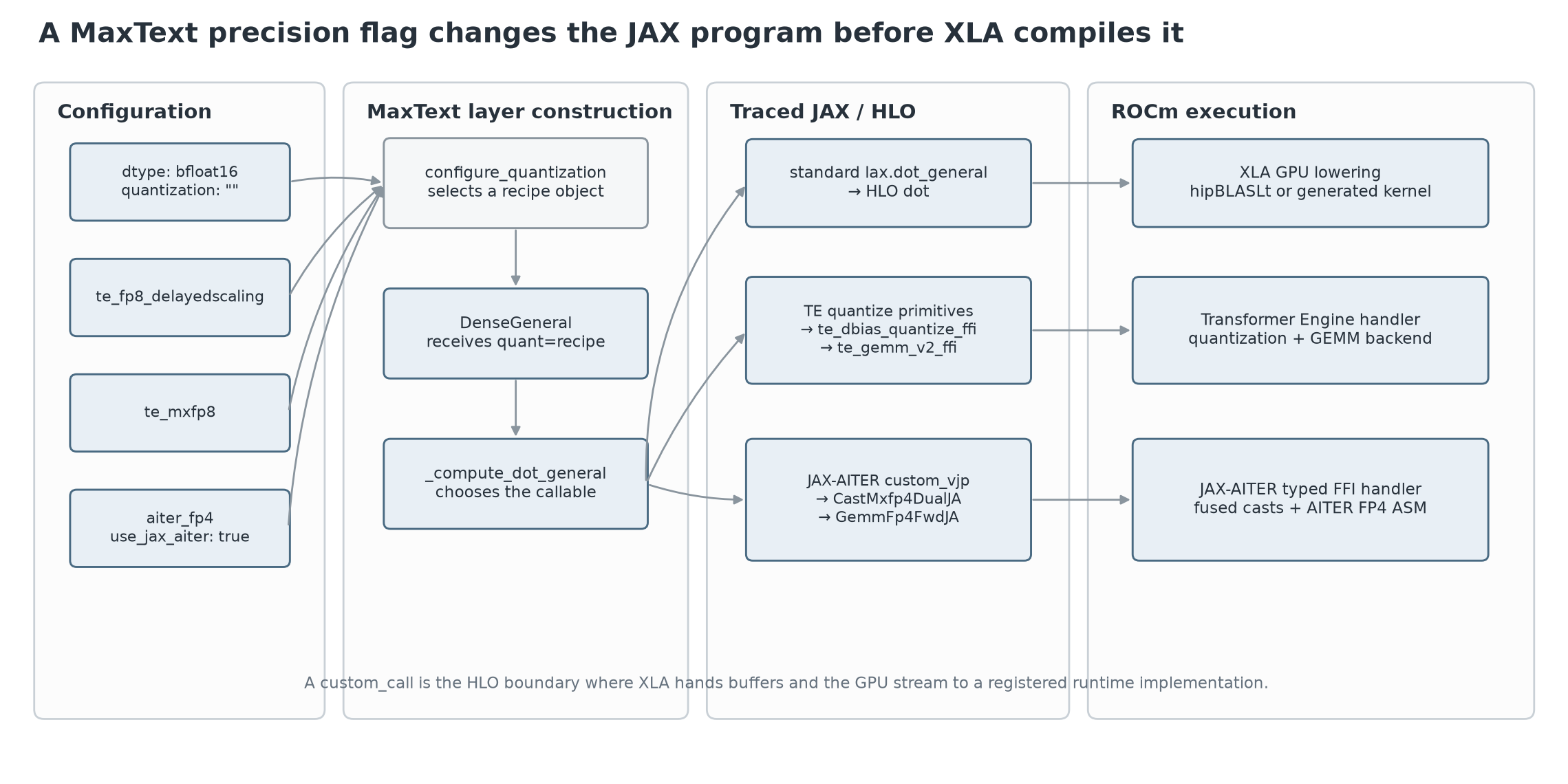
Eventually, a configuration choice must become a different JAX program. A YAML flag by itself cannot select a CDNA 4 matrix instruction; it must change the operations that JAX traces and lowers through XLA.
Dtypes and explicit quantize-dequantize
In the pinned JAX 0.11 source,
dtypes.py
exports float8_e4m3fn, float8_e5m2, float6_e2m3fn,
float6_e3m2fn, float4_e2m1fn, and float8_e8m0fnu from
ml_dtypes. A scalar dtype lets JAX
type-check values. It does not define a training recipe or guarantee a native
kernel for every operation and shape.
For per-tensor FP8, the representation can be written directly:
import jax
import jax.numpy as jnp

def quantize_fp8(x, dtype=jnp.float8_e4m3fn):
    qmax = jnp.asarray(jnp.finfo(dtype).max, jnp.float32)
    amax = jnp.max(jnp.abs(x.astype(jnp.float32)))
    scale = jnp.where(amax == 0, 1.0, amax / qmax)
    q = jnp.clip(x / scale, -qmax, qmax).astype(dtype)
    return q, scale

def fp8_dot(x, w):
    xq, sx = quantize_fp8(x)
    wq, sw = quantize_fp8(w)
    y = jax.lax.dot_general(
        xq, wq, (((xq.ndim - 1,), (0,)), ((), ())),
        preferred_element_type=jnp.float32,
    )
    return (y * sx * sw).astype(jnp.bfloat16)
This example is useful for a per-tensor forward GEMM. A training implementation must also define Dgrad, Wgrad, scale-state updates, sharding, and the backward rule.
An MX tensor is composite. Even when JAX exposes E2M1 as a scalar type, a
kernel-facing MXFP4 value needs packed element codes plus E8M0 scale arrays.
JAX-AITER’s pinned
gemm_fp4 wrapper
makes those buffers explicit:
call = jax.ffi.ffi_call(
    "GemmFp4FwdJA",
    jax.ShapeDtypeStruct((M, N), jnp.bfloat16),
    vmap_method="broadcast_all",
    has_side_effect=False,
)
out = call(a_packed, b_packed, a_scale, b_scale)
If a format has no suitable first-class array dtype, use this same pattern: store a packed integer payload and scale metadata, then pass both to a custom primitive or FFI call. Dequantizing to BF16 in ordinary JAX is useful for emulation, but native low-precision throughput requires a lowering that recognizes or directly consumes the packed representation.
MaxText chooses a JAX operation
MaxText keeps the surrounding computation dtype separate from quantization:
dtype: bfloat16
weight_dtype: float32
grad_dtype: float32
mu_dtype: float32
quantization: te_mxfp8
At ROCm/MaxText commit
b47d74bf,
configure_quantization
turns the string into an AQT, Flax FP8, or Transformer Engine recipe object.
DenseGeneral receives that object. Its
_compute_dot_general
contains the program-changing branch:
dims = ((axis, contract_ind), ((), ()))
dot_general = lax.dot_general
if quant:
    dot_general_cls = quant.dot_general_cls(mesh_axes=kernel_axes)
    dot_general = dot_general_cls()
    return dot_general(inputs, kernel, dims, precision=None)
return dot_general(inputs, kernel, dims, precision=matmul_precision)
The selected quantization recipe is injected into the model’s projection layers. As a result, changing a MaxText quantization setting changes the JAX operations emitted by those layers before compilation ever reaches XLA. Normalization, rotary embeddings, attention softmax, residual adds, and optimizer code remain separate JAX operations. Head coverage is branch- and recipe-specific.
The relevant recipe names in this environment are:
| MaxText value | Recipe selected | Scale state | HLO route |
|---|---|---|---|
quantization="" |
none | none | ordinary dot |
te_fp8_delayedscaling |
TE DelayedScaling |
FP32 scale + amax history | TE typed FFI |
te_fp8_currentscaling |
TE current per-tensor FP8 | current amax | TE typed FFI |
te_mxfp8 |
TE MXFP8BlockScaling |
E8M0 per 32 values | TE typed FFI |
aiter_fp4 |
JAX-AITER MXFP4, feature branch | packed E2M1 + E8M0 | JAX-AITER typed FFI |
The stock recipe mapping is pinned in
quantizations.py.
The MXFP4 experiment used ROCm/MaxText
b437942a,
where
aiter_fp4
installs a JAX-AITER-backed dot_general.
Transformer Engine and JAX-AITER
Transformer Engine sits between the model and the underlying GEMM
implementation. It receives high-precision tensors from MaxText, constructs
the low-precision operand representations required by the selected recipe,
and dispatches the corresponding GEMM implementation. In the measured
environment, the installed patched source is
6aa471b1.
For delayed FP8,
DelayedScalingQuantizeConfig
creates FP32 scale and amax-history state. For MXFP8,
BlockScalingQuantizeConfig
selects MXFP8_1D_SCALING without history. The GEMM primitive lowers to
te_gemm_v2_ffi,
carrying the data arrays, inverse scales, layouts, scaling mode, and output
dtype.
JAX-AITER provides a separate ROCm-native path. The Llama experiment pinned
35b7175c.
Its
gemm_fp4_bf16 implementation
uses a custom_vjp: Fprop consumes rowwise MXFP4 activation and weight
representations, Dgrad consumes the output gradient and columnwise weight, and
Wgrad consumes columnwise gradient and activation representations. The fused
cast target is CastMxfp4DualJA; the matrix target is GemmFp4FwdJA. The
registered
GemmFp4FwdJA handler
receives XLA’s ROCm stream and buffers, then launches an AITER FP4 assembly
kernel.
In HLO, custom_call means that XLA has reached this external operation
boundary. The target name selects a registered implementation; operands,
results, layouts, aliases, and attributes form its contract. The
JAX FFI guide covers the Python
interface, and the
OpenXLA custom-call documentation
defines the typed runtime ABI.
Precision changes in HLO
The following fixtures were captured on rocm:0 from JAX/JAXLIB 0.11.0,
MaxText b47d74bf, and Transformer Engine
2.17.0+6aa471b18. Each fixture uses a BF16 activation
[128,256], an FP32 master weight [256,256], and a BF16 output. The
compiled fixture was executed on MI355X. XLA emitted each DOT graph and
Graphviz rendered it after source-path tooltips were removed. Nodes, edges,
and visible labels are unchanged.
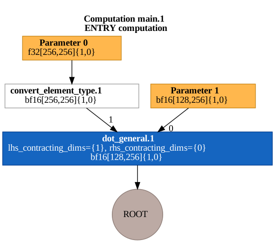
With no quantization object, MaxText’s branch casts the FP32 weight to BF16 and
emits an ordinary HLO dot:
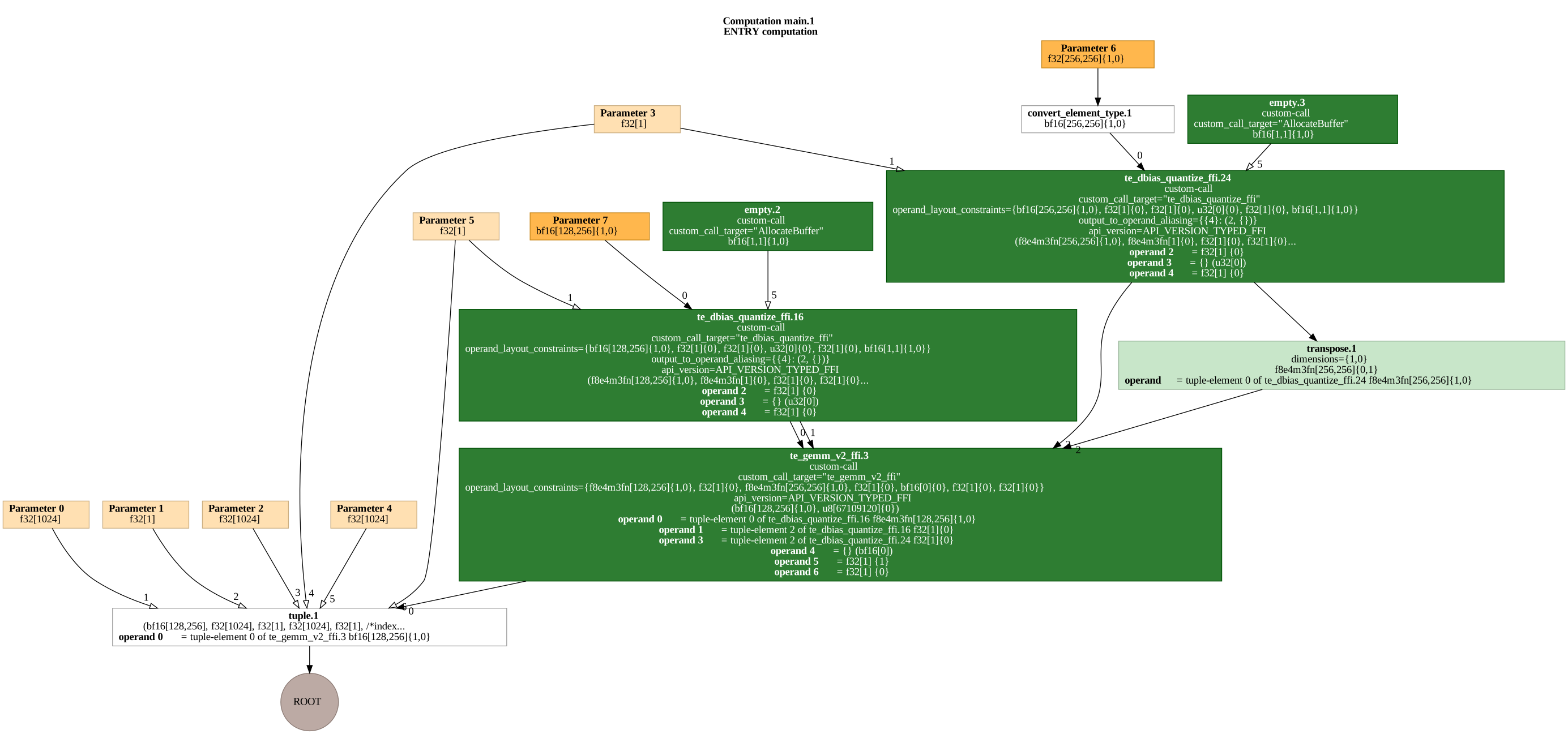
With quantization=te_fp8_delayedscaling, the recipe carries FP32 scale and
amax-history state. Each te_dbias_quantize_ffi receives the delayed scale;
its E4M3 arrays and per-tensor scales then enter te_gemm_v2_ffi, which
returns BF16:
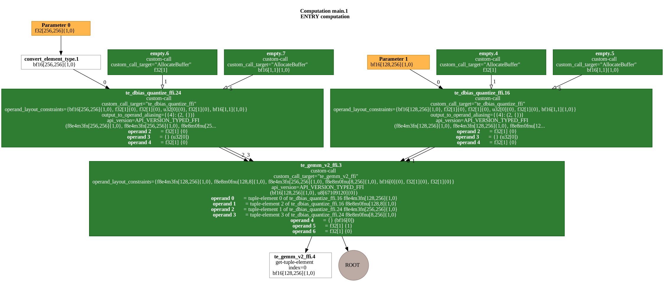
With quantization=te_mxfp8, the quantization calls return E4M3 arrays and
E8M0 scale arrays. The preserved HLO records
scaling_mode=MXFP8_1D_SCALING; the GEMM receives both data and scale
operands:
These graphs show the boundary visible to the compiler. Beyond the
custom_call, execution belongs to Transformer Engine, hipBLASLt, AITER, or
another backend implementation. Determining the exact kernel path requires a
runtime trace rather than HLO alone.
Case study: Llama 2 70B
The case study compares five timed configurations under one training-step protocol.
Configuration and recipes
| Item | Value |
|---|---|
| Hardware | 8× MI355X, one node |
| Parallelism | FSDP-8 |
| Model | MaxText llama2-70b |
| Sequence length | 4,096 |
| Global batch | 120 sequences |
| Tokens per update | 491,520 |
| Local batch | 15 sequences per GPU |
| Attention | Transformer Engine fused attention |
| Rematerialization | full |
| Timed window | post-warmup steps 10–29 of 30 |
| Input | reused synthetic batch |
All low-precision arms keep weight_dtype, grad_dtype, and the Adam moment
dtypes in FP32. The surrounding computation is BF16 except in the FP16 arm.
| Arm | Surrounding dtype | Projection recipe |
|---|---|---|
| BF16 | BF16 | ordinary MaxText dot_general |
| FP16 | FP16 | ordinary MaxText dot_general |
| FP8 | BF16 | TE per-tensor delayed scaling |
| MXFP8 | BF16 | TE E8M0 block scaling over 32 values |
| MXFP4 | BF16 | JAX-AITER MXFP4 for MLP, Q/K/V/O, and logits projections; fused attention core remains BF16 |
The MXFP4 distinction is explicit in its launcher:
quantization: aiter_fp4
use_jax_aiter: true
aiter_attention: false
The launcher also sets AITER_FP4_MLP=1 and AITER_FP4_ATTN=1.
AITER_FP4_ATTN=1 covers the Q/K/V/O linear projections.
aiter_attention=false leaves the fused attention core on the Transformer
Engine BF16 path.
The BF16, FP16, FP8, and MXFP8 arms use stock ROCm/MaxText v26.6 at
b47d74bf. MXFP8 uses the patched Transformer Engine revision cited above.
The MXFP4 arm uses the pinned ROCm/MaxText feature revision and JAX-AITER
alpha2 source.
Expectations before results
The raw peak ratios suggest $r=2$ for FP8/MXFP8 and $r=4$ for MXFP4 relative to BF16. Let $f$ be the fraction of baseline step time spent in eligible GEMMs, and assume those GEMMs improve exactly by $r$ while all other time is unchanged. Amdahl’s law gives
\[S_{\mathrm{step}}(f,r) =\frac{1}{(1-f)+f/r}.\]Chapter 3 did not supply a measured eligible-GEMM fraction for this exact Llama run, so $f$ remains an assumption. The table spans 70%, 80%, and 90%; it does not infer $f$ from the measurements.
| Assumed eligible time $f$ | FP8/MXFP8, $r=2$ | MXFP4, $r=4$ |
|---|---|---|
| 0.70 | 1.54× | 2.11× |
| 0.80 | 1.67× | 2.50× |
| 0.90 | 1.82× | 3.08× |
FP16 has $r=1$ from the published peak, so this model predicts 1.00× for every $f$. Any FP16/BF16 timing difference comes from realized kernels, layouts, or surrounding work rather than a higher advertised matrix ceiling. The Amdahl table is optimistic about conversion and scale overhead.
Throughput is only one reason to use lower precision. The second question is whether these formats meaningfully reduce memory usage.
Let $P$ be the parameter count, $N_F$ the FSDP degree, $A_h$ the number of saved elements that stay BF16, and $A_e$ the number eligible for a lower-precision saved representation. With FP32 master weights, gradients, and two Adam moments:
\[\begin{aligned} M_{\mathrm{persistent}} &=\frac{P}{N_F}(4_{\mathrm{master}}+4_m+4_v),\\ M_{\mathrm{gradient}} &=\frac{P}{N_F}(4_g),\\ M_{\mathrm{saved}} &=2A_h+A_e\left(\frac{b}{8}+\frac{s}{k}\right),\\ M_{\mathrm{expected}} &=M_{\mathrm{persistent}}+M_{\mathrm{gradient}} +M_{\mathrm{saved}}+M_{\mathrm{workspace}}. \end{aligned}\]For nominal $P=70$ billion and $N_F=8$, persistent FP32 parameters and moments use about 105 GB per GPU; one FP32 gradient shard adds about 35 GB. Quantizing GEMM operands does not change those 140 GB. Additional savings apply only when the converted representation is saved or transferred; an on-the-fly conversion at the GEMM changes operand and workspace live ranges.
For a full MX block, $k=32$ and $s=1$ byte. The eligible saved-tensor term is:
| Saved representation | Bytes per eligible element | Fraction of BF16 payload |
|---|---|---|
| BF16 | 2.0000 | 1.000 |
| per-tensor FP8 | about 1.0000 | 0.500 |
| MXFP8 | 1.03125 | 0.516 |
| MXFP6 | 0.78125 | 0.391 |
| MXFP4 | 0.53125 | 0.266 |
This predicts storage for identified tensors, not peak process HBM. Peak HBM also depends on rematerialization, live ranges, FSDP all-gathers, compiler temporaries, row/column copies, and backend workspaces. The JAX Scaling Book training chapter uses the same separation between sharded parameters, optimizer state, and activation checkpoints.
Train-step results
Job 124490 measured post-warmup steps 10–29. The values below are copied from the captured result bundle. The expected column uses the Amdahl model above with an 80% eligible-GEMM time share.
| Precision | Mean step | Std dev | TFLOP/s/device | Tokens/s/device | Expected speedup | Measured speedup |
|---|---|---|---|---|---|---|
| BF16 | 27.028 s | 0.107 s | 973.8 | 2,273.2 | 1.00× | 1.00× |
| FP16 | 25.110 s | 0.082 s | 1,048.2 | 2,446.9 | 1.00× | 1.08× |
| FP8 | 15.006 s | 0.044 s | 1,754.0 | 4,094.4 | 1.67× | 1.80× |
| MXFP8 | 17.838 s | 0.180 s | 1,475.7 | 3,444.8 | 1.67× | 1.52× |
| MXFP4 | 11.704 s | 0.038 s | 2,248.8 | 5,249.5 | 2.50× | 2.31× |
Tokens/s/device follows
\[\mathrm{tokens/s/device} =\frac{491{,}520}{8\,t_{\mathrm{step}}},\]using the unrounded step samples in the result bundle. MaxText reports TFLOP/s/device from its model-operation estimate divided by step time; it is not a count of issued MFMA instructions.
The measured results broadly follow the expected trend. FP8 delivers a 1.80× speedup, near the upper end of the range predicted by the simple Amdahl model. MXFP8 improves throughput by 1.52×, suggesting that scale handling, conversion overhead, and realized kernel performance consume part of the theoretical gain. MXFP4 achieves a 2.31× speedup, substantially faster than FP8 while remaining within the range predicted by the model.
The broader lesson is that lower-precision formats can substantially accelerate training, but realized speedups are bounded by the fraction of execution time spent inside the accelerated GEMMs. The matrix peak provides the opportunity; the rest of the training step determines how much of that opportunity can be realized.
The artifact does not contain an MFU field. A single peak denominator would mislabel these mixed-operation recipes, so the table keeps the captured model-TFLOP/s values rather than synthesizing MFU.
From precision to memory placement
The Llama case keeps roughly 105 GB per GPU of sharded FP32 parameters and Adam moments before gradients, activations, all-gathers, and workspaces. Choosing FP8 or MXFP4 for projection operands does not decide where those remaining bytes live or when they are materialized.
Chapter 5 starts from this memory equation. It maps global tensors onto a device mesh, derives the resulting local shapes and collectives, and compares FSDP with expert parallelism. Chapter 6 then applies rematerialization and kernel choices to those local operations.