Profiling a Training Step

Chapter 3 of How to Scale Your Model on AMD (Chapter 2: The JAX/ROCm Stack | Chapter 4: Training in Mixed Precision)

How to measure a JAX training step on MI355X, attribute GPU work through XSpace and HLO, and validate kernels with ROCprofiler-SDK counters.

A training step can be viewed at several different layers of abstraction.

At the framework level, we care about which part of the model consumed time. At the compiler level, we care about which HLO operations were generated. At the runtime level, we care about which kernels and collectives actually executed.

Ideally, a profiler should connect these views:

1. the duration and throughput of one optimizer update;
2. the JAX or MaxText component that requested the work;
3. the optimized HLO that XLA compiled; and
4. the HIP kernel or RCCL operation that ran on the GPU.

Current, different profilers operate stronger at different levels. Framework and compiler attribution are most visible through XPlane and XProf, while runtime execution is most directly observed through ROCm profiling tools. Taken together, they provide a path from model code to generated HLO and ultimately to the kernels and collectives that executed on the GPU.

Hardware counters form a separate layer of evidence. Because dispatch-level counter collection alters the execution schedule, counters are typically collected in a focused run after the relevant kernels have already been identified.

Profiler metrics

Before opening a profiler, define exactly what is being measured. Most performance disagreements originate from mismatched definitions rather than incorrect measurements.

In this chapter, one train step is one optimizer update. If gradient accumulation is two, the step contains two forward/backward microsteps and one optimizer update. Compilation, checkpointing, evaluation, and data-loader stalls are reported separately unless the experiment is explicitly measuring end-to-end job time.

End-to-end metrics

The most common training metrics appear simple, but each depends critically on its denominator.

Global tokens/s is the input token count divided by synchronized step time; per-device tokens/s divides that value by the number of accelerators. MFU uses the declared useful model FLOPs and the matching per-device compute peak:

\[\mathrm{MFU} =\frac{F_{\mathrm{model}}} {G\,t_{\mathrm{step}}\,C_{\mathrm{peak}}}.\]

MaxText defines MFU from theoretical model FLOPs and measured step time. This distinction is intentional. Useful model FLOPs measure algorithmic work, whereas executed FLOPs measure everything the hardware actually performed. The difference becomes important once rematerialization, routing, padding, and communication are introduced.

Metric	Required denominator	Report with it
Step time	one synchronized optimizer update	warmup window, statistic, spread
Tokens/s	global input tokens in that update	global or per-device; padded or non-padding
Useful MFU	declared useful model FLOPs	dtype peak, device count, FLOP ledger
Executed FLOP rate	operations actually executed	kernel/component boundary and evidence source
Memory footprint	bytes on one physical GPU	static compiled peak, observed high-water mark, worst device
Component time	union of attributed device intervals	device/rank, step, overlap rule

These definitions eliminate a number of surprisingly common benchmarking mistakes:

• Do not multiply a resolved global batch by the device count again.
• Do not count top-$k$ expert assignments as input tokens. Assignment throughput is a separate metric equal to $kN_{\mathrm{tok}}/t$ before drops.
• Use the dense BF16 peak for dense BF16 MFU. A structured-sparse or FP8 peak is valid only when the measured kernels use that path.
• Report the maximum per-device memory footprint. Summing HBM across devices does not show whether one shard fits.
• Do not call one observed duration a median. A stable timing result needs several post-warmup updates and a dispersion statistic.

Another common source of confusion is JAX’s asynchronous execution model. Compile and autotune before the retained timing window, then call jax.block_until_ready() at its boundaries.

Profiling runs should explain performance, not define it. Final throughput numbers should come from an otherwise identical workload running without profiling overhead.

Memory usage also has both a static and a dynamic interpretation. XProf’s Memory Viewer uses compiler data to show the static buffer assignment and its peak in program order. The dynamic Memory Profile and device telemetry show allocator behavior at runtime. Record arguments, outputs, aliases, temporaries, and runtime high-water marks rather than collapsing unlike values into one unexplained number.

Roofline analysis

Roofline analysis provides a simple way to reason about whether a workload is limited by computation or data movement. The JAX Scaling Book roofline chapter introduces the plot below. Arithmetic intensity is the work performed per byte moved, $I=F/Q$. For peak compute $C$ and bandwidth $\beta$, the roofline is

\[P_{\mathrm{roof}}=\min(C,I\beta).\]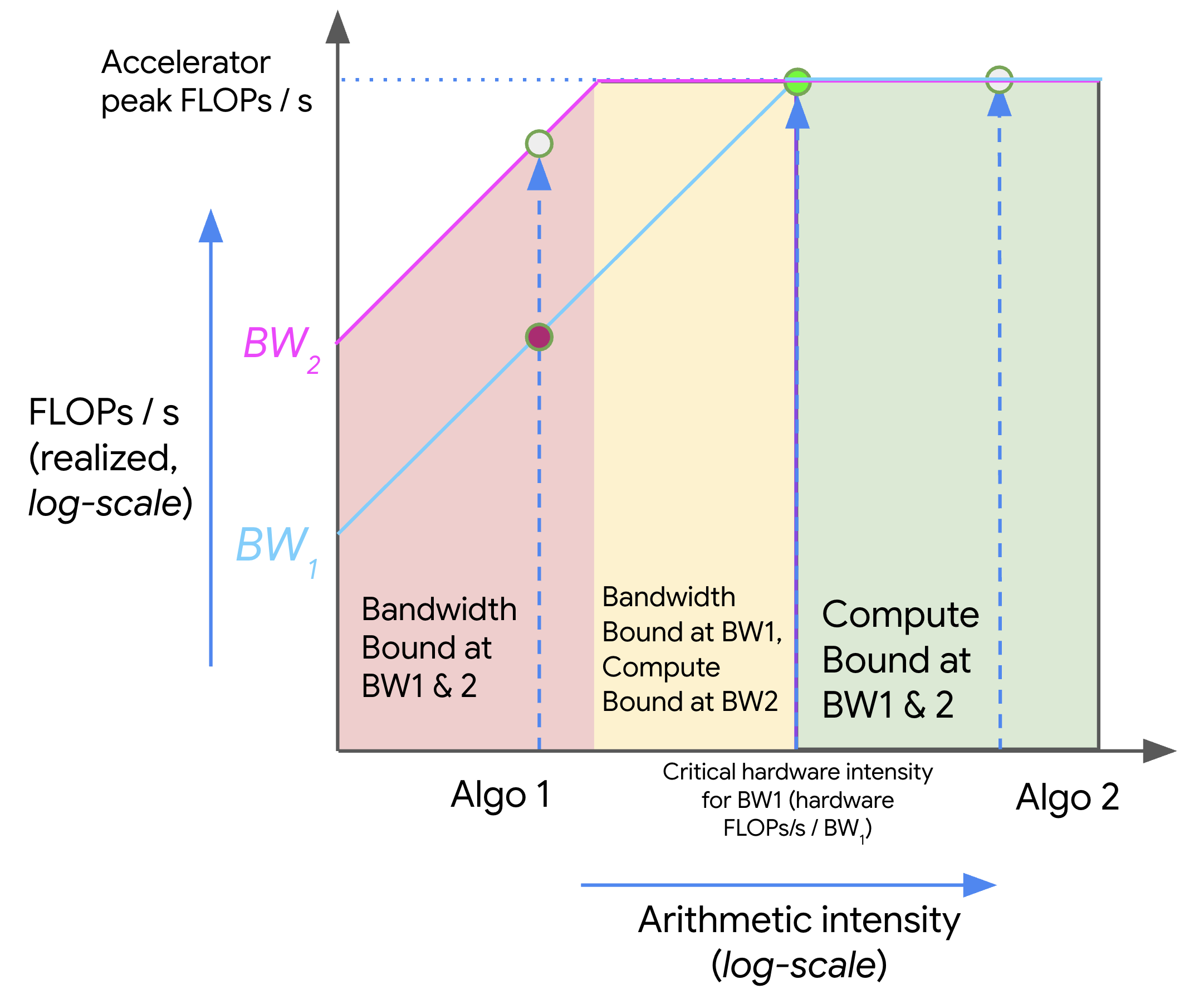

The generic roofline from the MIT-licensed JAX Scaling Book. Its BW1 and BW2 lines illustrate two memory systems or two achieved bandwidths. The MI355X values are substituted in the text rather than drawn into the source figure.

The source chapter applies this diagram to TPU v5e. For one full MI355X in SPX mode, the dense BF16 matrix ceiling is 2.5166 PFLOP/s and HBM bandwidth is 8 TB/s, so the BF16/HBM ridge is about 315 FLOP/byte. The ridge point divides two fundamentally different optimization regimes. To the left, reducing memory traffic matters most. To the right, increasing computational efficiency becomes the dominant concern.

A roofline is only meaningful if the bandwidth term matches the memory system being analyzed. An HBM roofline counts HBM traffic; an L1/LDS roofline counts traffic at that level; a network roofline uses collective payload and link bandwidth. For a component, sum the executed FLOPs and measured bytes of its kernels, then divide by the union of its device intervals so overlapping streams are not counted twice.

The JAX profiler

The JAX profiler is the highest-level profiling interface used throughout this book. jax.profiler.start_trace is its Python entry point. The implementation combines host instrumentation, backend-specific device events, and compiler sideband data. XProf then derives higher-level views from those sources.

XLA profiler backend

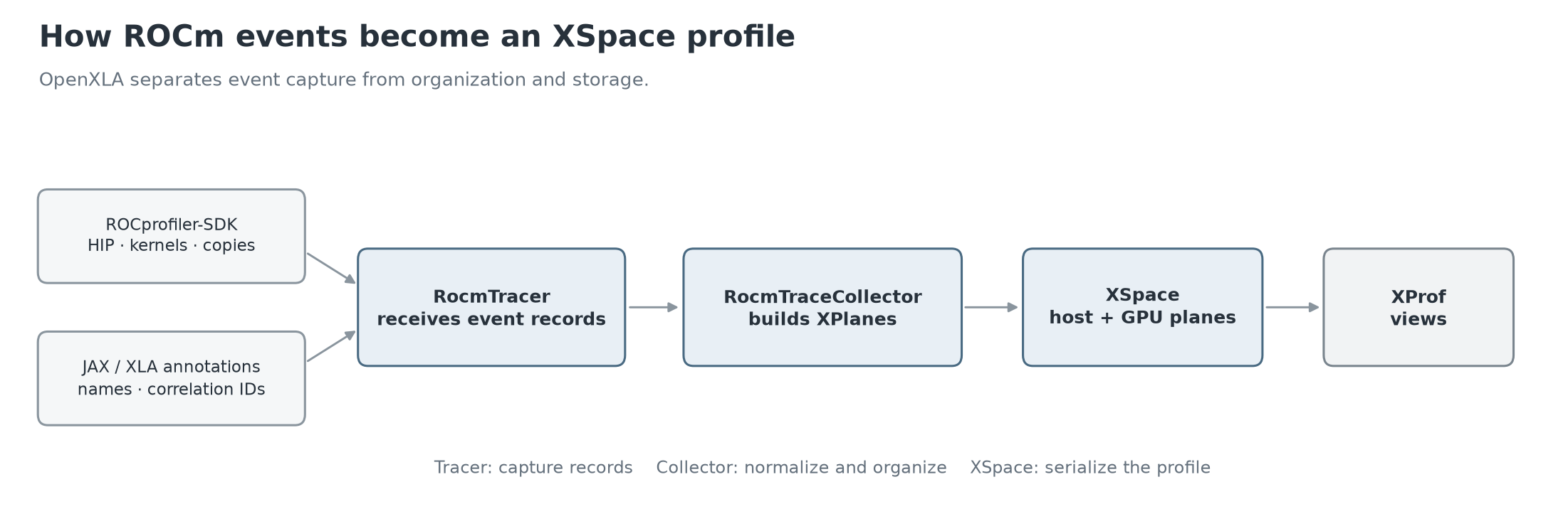
Internally, profiling begins when JAX asks OpenXLA to create a ProfilerSession. On ROCm, two components are particularly important:

• RocmTracer configures ROCprofiler-SDK and receives HIP API, kernel-dispatch, and memory-copy records. Correlation IDs and the active JAX/XLA name stack travel with those records.
• RocmTraceCollector normalizes timestamps and writes the events and metadata into host and GPU XPlanes.

The result is a single profiling artifact that combines framework information, compiler metadata, and GPU execution records. This artifact is an XSpace, which XProf reads.

The JAX profiler path. Python starts a session, the XLA profiler backend populates an XSpace protobuf, and XProf parses that schema into timeline, roofline, kernel-statistics, and framework-op views.

XSpace

XSpace is the storage format used by XProf and OpenXLA profiling tools. Conceptually, it is a hierarchy of planes, lines, events, and metadata.

The authoritative xplane.proto defines the hierarchy. An XSpace contains XPlanes for hosts, devices, and sideband data. Each plane contains parallel XLines, each timed interval is an XEvent, and XStats hold fields such as correlation ID, HLO name, kernel geometry, and source metadata.

An XSpace as displayed by XProf. The screenshot labels a displayed timeline as an XLane; the protobuf message is named `XLine`. XEvents occupy intervals on a line, and the selected event's XStats appear in the details pane.

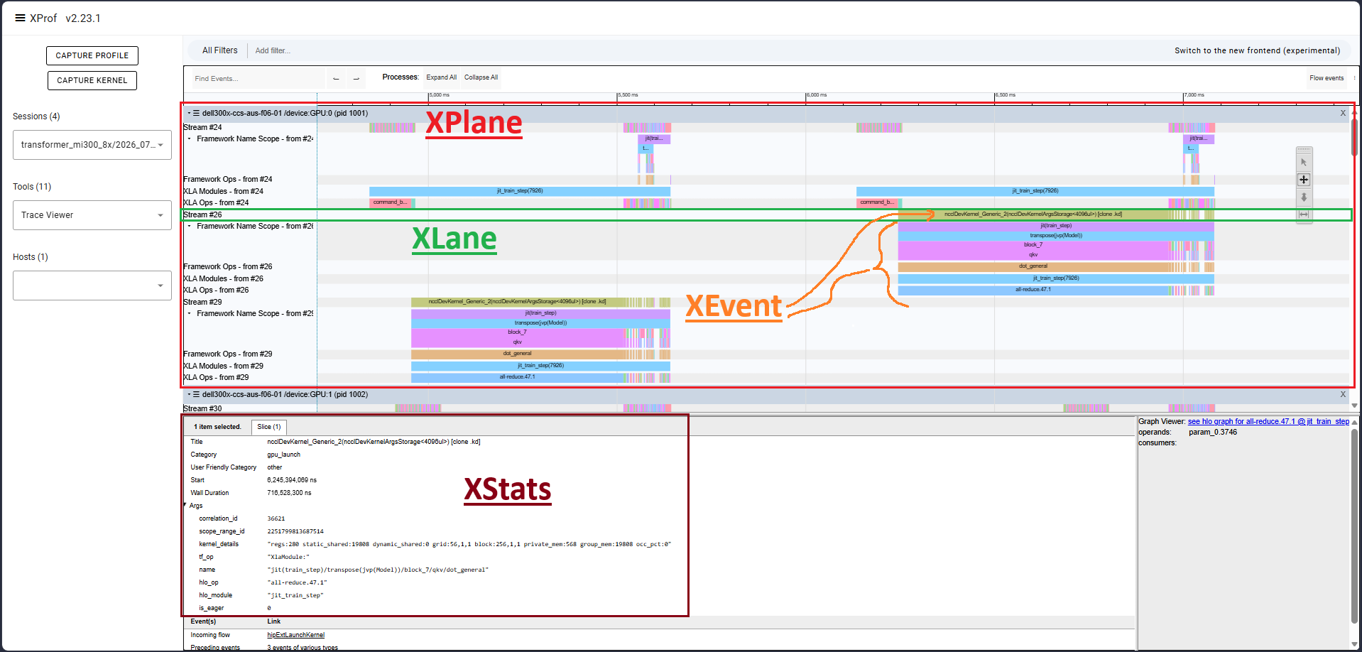
XProf’s GPU lines must be read with this distinction in mind. The Trace Viewer documentation states that raw GPU stream data is directly grounded in the collected profile, while GPU XLA-op and framework lines are derived from stream data and optional compiler metadata. This distinction matters because compiler operations and runtime kernels rarely map one-to-one. A single HLO operation may generate multiple kernels, while the same kernel implementation may be reused by many HLO operations.

XProf

The JAX Scaling Book profiling chapter introduces the generic XProf workflow. This section focuses specifically on the XProf views that are most useful for model-performance investigations. The official XProf documentation covers Overview, Trace Viewer, HLO Op Stats, Graph Viewer, Memory Viewer, and exports. Start a local instance against the retained log directory:

python -m pip install xprof
xprof --logdir="$PROFILE_DIR" --port=6006

On MI355X, first confirm that GPU stream lines are present, the device is identified as gfx950, and the selected interval contains complete post- warmup steps. A host-only trace cannot support kernel or GPU roofline claims.

GPU Kernel Stats

GPU Kernel Stats groups each unique kernel and originating framework-operation pair. Its most useful columns are kernel name, op name, occurrences, total/average/minimum/maximum duration, register count, shared-memory use, block and grid dimensions, and occupancy when available.

A practical investigation typically proceeds in the following order:

1. Sort by total duration to find the kernel/op pairs that dominate the capture.
2. Filter by an existing MaxText scope such as wi_0, attention, or combine.
3. Check occurrences against layers, gradient-accumulation microsteps, and forward/backward expectations.
4. Follow the op name into HLO. Record every emitted kernel, including transposes, reductions, and epilogues around the main GEMM.
5. Match the full or stable kernel-name prefix in the rocprofv3 trace.

Avoid assuming that a row corresponds directly to a model-layer operation. One HLO fusion can emit several kernels, and the same library kernel can serve several HLO operations.

GPU roofline analysis

XProf’s Roofline Model supports GPU profiles in beta. It can show program-level and operation-level points for HBM and L1/shared memory. The page may expose both XLA cost-model FLOP rates and rates derived from hardware counters. Keep those labels in exported data; they are different evidence.

Before reporting any roofline efficiency number, verify the assumptions used to construct the roofline itself.

• verify the Device Information peaks against the captured MI355X partition, dtype, and clock convention;
• identify whether FLOPs and bytes are compiler estimates or counter-derived;
• filter to one component and inspect the operations omitted by that filter;
• compare operation points with GPU Kernel Stats because HLO-to-kernel attribution is many-to-many; and
• recompute the point from retained rows if the device peak or byte level is wrong.

A visually impressive roofline point is meaningless if the ceilings, FLOPs, or bandwidth measurements are wrong. In particular, do not apply one BF16 peak to FP32 router reductions, FP8 GEMMs, and RCCL kernels.

rocprofv3

rocprofv3 is the command-line client built on ROCprofiler-SDK. Use rocprofv3 only after XProf has narrowed the investigation to a specific step, component, or HLO operation.

Trace collection

Run the same resolved MaxText configuration in a fresh process with its JAX profiler disabled:

rocprofv3 \
  --runtime-trace --rccl-trace \
  --output-directory "$ROCPROF_DIR" \
  --output-format rocpd -- \
  python -m maxtext.trainers.pre_train.train "$CONFIG" \
    run_name=profile-rocprof profiler="" steps=14

--runtime-trace collects HIP runtime, marker, kernel-dispatch, and memory activity; --rccl-trace makes the collective requirement explicit. Keep the default rocpd database. AMD recommends converting rocpd after collection because direct CSV and PFTrace output can omit newer record types:

rocpd convert -i "$ROCPROF_DIR/<pid>_results.db" \
  --output-format pftrace

The purpose of the runtime trace is to answer questions that compiler artifacts cannot answer. It shows which HIP calls launched work, which queues carried kernels, whether kernels overlapped, when memory copies occurred, and where RCCL activity was exposed. Correlation IDs connect host APIs to asynchronous dispatch records.

When analyzing GPU execution, dispatch timestamps matter more than host API durations. Kernel start and end timestamps define device execution time, whereas the HIP API duration describes host-side launch activity.

Like all profiling tools, tracing perturbs the program being observed. Use it to explain the matched unprofiled timing, not to replace it.

Without profiler-control instrumentation, this command also records startup and warmup; select complete steps 10–12 during analysis. If the application has a thin ROCTx control hook, add --selected-regions, resume immediately before step 10, synchronize after step 12, and then pause. That reduces the trace without changing the compiled train-step body.

Perfetto

Perfetto provides the most direct view of runtime execution. Open the converted trace in Perfetto UI. For one complete step:

1. pin the host step or ROCTx track;
2. pin the selected GPU’s compute and copy queues;
3. show RCCL API and RCCL kernel tracks;
4. zoom to the exact step boundaries;
5. select the candidate dispatch and record its kernel name, queue, start, duration, correlation ID, grid, workgroup, LDS, scratch, and register data;
6. measure interval unions for components and intersection intervals for overlap.

A common mistake is to sum durations across devices and compare the result to wall-clock time. Choose the critical rank/device, or report per-device values and their spread.

ROCTx annotations

ROCTx is best viewed as a host-side annotation system rather than a device-side tracing mechanism. It provides markers, push/pop ranges, and profiler pause/resume control. With rocprofv3 --selected-regions, collection starts disabled and occurs only between roctxProfilerResume(0) and roctxProfilerPause(0). Place the pause after a device synchronization so queued work is not cut off.

The most important limitation is that ROCTx cannot divide a single compiled JAX executable into internal GPU regions. Python inside a jax.jit function runs while JAX traces the function, not for every execution. A ROCTx call around the outer Python invocation can bracket the whole synchronized step, but it cannot divide that executable into attention, router, and expert device ranges. jax.named_scope plus optimized HLO supplies that internal attribution.

For non-jitted code or a program that intentionally launches several compiled executables, host ROCTx ranges can bracket each launch. Synchronize within the range when the range is meant to cover device completion. Attribution should follow the program’s natural structure rather than being distorted to improve trace readability.

When a JAX/XLA build exports direct application ROCTx events into XSpace, they appear as host marker lines. They remain host ranges; their presence does not turn them into device-side annotations.

PMC collection

Performance counters provide the lowest-level evidence used in this chapter. ROCprofiler-SDK collects performance monitoring counters (PMCs) at dispatch level. List and validate the counters provided for the installed gfx950 stack:

rocprofv3-avail list --pmc
rocprofv3-avail pmc-check SQ_WAVES GRBM_GUI_ACTIVE

Then filter to a stable kernel name and occurrence:

rocprofv3 \
  --pmc SQ_WAVES GRBM_GUI_ACTIVE \
  --kernel-include-regex '<escaped-kernel-prefix>' \
  --kernel-iteration-range 10-10 -- \
  python kernel_replay.py

The example counters demonstrate workflow only; meaningful analysis requires architecture-specific FLOP, bandwidth, cache, occupancy, or stall metrics. Select them from rocprofv3-avail, and record the formulas used to turn raw counters into bytes or operations.

The ROCprofiler-SDK counter service requires serialized kernel execution for per-dispatch counting. Streams and queues retain their identities, but kernels on the target GPU no longer run concurrently. This design has several important consequences:

• PMC durations do not measure the production schedule or overlap;
• co-dependent kernels can deadlock under dispatch serialization;
• multiple --pmc groups run separate application passes; and
• counters from different passes are comparable only when the selected dispatch, shape, route, and launch configuration repeat.

Runtime traces answer timing questions. PMCs answer hardware-behavior questions. Treat those as complementary rather than interchangeable forms of evidence.

TraceLens

AMD TraceLens can read JAX XPlane, rocprofv3 JSON, and PFTrace data and generate structured performance reports. Its official JAX report guide provides:

TraceLens_generate_perf_report_jax \
  --profile_path "$XPLANE"

TraceLens should be treated as a convenience layer rather than a primary source. The current compatibility matrix pins xprof==2.20.1 and protobuf>=6.31.1,<7, while the inspected JAX 0.11 MaxText environment contains XProf 2.23.1. Run TraceLens in a separate environment, retain the generated tables, and validate its categories against XProf, HLO, and raw runtime records. It does not replace those primary sources.

rocprof-compute

rocprof-compute is designed for deep investigation of individual kernels rather than full training steps. It collects predefined counter groups and derives kernel-level analyses. Start from a kernel name and launch configuration found in the normal trace, then prefer a deterministic single-kernel reproducer:

rocprof-compute profile \
  --output-directory "$PROFILE_OUTPUT" \
  --kernel 'stable_kernel_name_substring' \
  --dispatch 1 -- \
  python expert_replay.py

rocprof-compute analyze \
  --path "$PROFILE_OUTPUT" \
  --experimental --gui

Profile mode can replay the application many times to collect incompatible counter groups. Kernel and dispatch filters reduce that cost. Replaying a full distributed MaxText job also repeats initialization and can make dispatch IDs unstable, so extraction is preferable. Iteration multiplexing avoids application replay by spreading counter groups over repeated dispatches, but it needs enough identical occurrences and trades accuracy for collection speed.

The analysis combines top kernel statistics, speed-of-light metrics, memory and cache behavior, and an empirical roofline. The reported timings describe the replay experiment, not end-to-end training performance.

Worked example: profiling a Mixtral 8x22B training step

The remainder of the chapter applies the profiling workflow to a concrete Mixtral 8x22B training configuration.

The configuration uses case-study source commit a32b51d6 and MaxText’s mixtral-8x22b.yml at the inspected ROCm MaxText v26.6 commit b47d74bf. It matches the main architecture facts published by Mistral AI.

Quantity	Value
Decoder layers	56
Model width $D$	6,144
Query heads / KV heads	48 / 8
Head dimension	128
Expert width $F$	16,384
Experts / selected experts	8 / 2
Vocabulary	32,768
Sequence length	4,096
Per-device batch / accumulation	4 / 2
Devices / mesh	8 MI355X / FSDP=4, EP=2
Global tokens per update	262,144
Dtype	BF16

Here $4\times8\times2=64$ sequences contribute to an update, so $N=64\times4096=262{,}144$ input tokens.

The experiment requests Transformer Engine fused attention, scanned layers, and save_dot_with_context_except_mlp rematerialization. It uses a synthetic batch and performs two forward/backward microsteps before each AdamW update.

Decomposing a train step

Before attributing time, divide the training step into meaningful computational stages.

One optimizer update contains two accumulation microsteps. Each microstep has a forward pass through the embedding, 56 decoder layers, final norm, language model head, and loss, followed by the corresponding reverse-mode work. The optimizer runs once after gradients from both microsteps have accumulated.

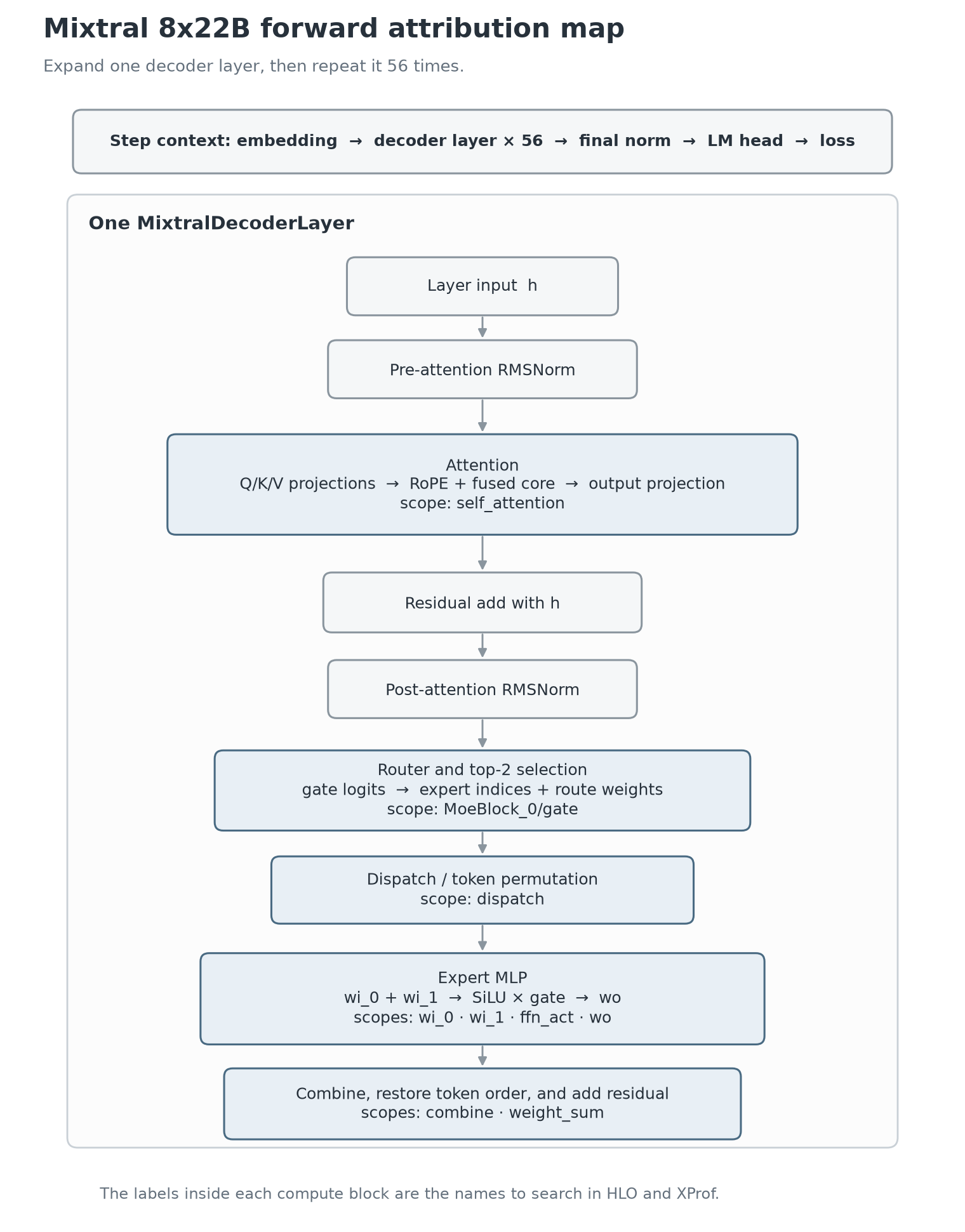
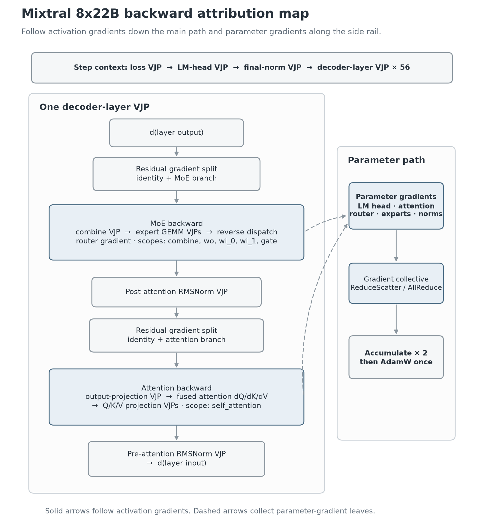
Within a decoder layer, attribute attention, routing, token movement, expert compute, normalization, and residual work separately. The next two diagrams give those forward and backward boundaries.

Forward pass

From a profiling perspective, the forward pass consists of two dominant subsystems: attention and expert computation.

MaxText’s MixtralDecoderLayer applies pre-attention RMSNorm, grouped-query self-attention, an attention residual, post-attention RMSNorm, and a routed MoE block. The router selects two of eight experts for each token. The selected routes become dispatch and combine masks in this fixed-capacity configuration. Tokens enter two expert input projections (wi_0, wi_1), combine through SiLU gating, pass through wo, and return to token order under the route weights. The existing scope names come from the same release’s RoutedMoE.

One decoder layer expanded into a single top-to-bottom flow. The highlighted blocks include the MaxText scope names used to correlate model regions with HLO and XProf; the forward attribution table below uses these boxes as its accounting categories.

Backward pass

The backward pass should be treated as a separate computational workload rather than a mirror image of the forward pass. Automatic differentiation produces input-gradient and weight-gradient GEMMs, reduction and transpose fusions, the fused-attention backward implementation, reverse token movement, router gradients, and gradient collectives. Custom VJPs can replace the default transpose rules.

Rematerialized forward work executes inside the backward interval. Attribute that device time to backward/rematerialization while keeping the useful model FLOP ledger unchanged.

Activation gradients follow the vertical decoder-layer VJP. Parameter gradients from the MoE and attention branches feed the side rail for collectives, microstep accumulation, and the optimizer update. The backward attribution table below treats parameter-gradient work as part of its originating VJP rather than counting the side rail twice.

Time attribution in JAX

The forward and backward diagrams define semantic components. Turning those components into times requires an exclusive accounting rule so that one kernel is not charged to several boxes.

For a standalone JAX model, place named_scope around the components before applying value_and_grad and jit, then place one StepTraceAnnotation around the synchronized optimizer update. Attribute a captured step in this order:

1. Select one complete step on one GPU.
2. Remove collective kernels into a communication bucket before classifying model work.
3. Within the backward interval, classify checkpoint/rematted_computation as replayed forward work before assigning the remaining transpose(jvp(...)) operations to gradient computation. Use jvp(...) for forward work and the code outside the model VJP for loss, gradient accumulation, and the optimizer.
4. Within each phase, use the deepest stable named_scope to assign a component. Keep operations whose metadata was lost in an explicit unattributed bucket.
5. With a raw XPlane, merge the event intervals in each component and reconcile their union with the step boundary. Summed kernel durations are a different quantity and can exceed wall time when streams overlap.

Named scopes assist attribution, but they do not define execution boundaries. A residual add may disappear into an adjacent fusion, while one named projection may emit several kernels. Confirm each large bucket against its HLO shapes and runtime kernel names.

For this case study, the missing profile was generated directly on the local eight-MI355X system. The instrumented source is MaxText b47d74bf with metadata-only jax.named_scope labels around the map components, gradient-accumulation loop, loss, and optimizer. These labels do not change array values or shardings.

The capture uses the 8x22B FSDP=4/EP=2 configuration above. It records one complete step after compilation and two preceding steps on eight MI355X GPUs. The profiled step took 20.605 seconds; the adjacent steady steps took 20.824 and 20.811 seconds.

Kernel Stats aggregates every occurrence on all eight GPUs. The component tables therefore report mean summed HLO self-time per GPU-step, obtained by dividing those aggregates by eight. Raw stream intervals provide the separate wall-time and overlap calculation.

Exclusive phase bucket	Mean device time	Share of summed device time
Forward model compute	2,322.8 ms	8.7%
Backward gradient compute	7,287.9 ms	27.3%
Rematerialized forward replay	2,210.5 ms	8.3%
Loss, gradient accumulation, and named optimizer work	9.5 ms	<0.1%
Communication	14,560.8 ms	54.6%
Unattributed work	297.5 ms	1.1%
Total summed device time	26,689.0 ms	100%

The summed total exceeds wall time because computation and communication overlap. Across the eight raw GPU timelines, the mean compute union is 12.128 seconds and the mean communication union is 14.561 seconds. Their intersection is 5.966 seconds, leaving 8.594 seconds of exposed communication:

\[12.128 + 14.561 - 5.966 = 20.723\ \mathrm{s}.\]

The resulting busy union is 20.723 seconds inside a 20.759-second device-event span, leaving 36 ms with no GPU work. The event span and the logged 20.605-second step use slightly different profiler boundaries, so the component tables reconcile to the raw device timeline rather than to the host log.

Time attribution in MaxText

MaxText already exposes a useful attribution vocabulary through its existing scope names. The forward table groups those names into the boxes in the forward map. Attention combines the Q/K/V/O projections, RoPE/layout work, and fused core; Expert MLP combines wi_0, wi_1, ffn_act, and wo.

The retained extraction script classifies each Kernel Stats row exactly once and emits the machine-readable ledger used for these tables. It uses the phase name stack first and then the explicit component scope. Rows without phase metadata remain unattributed. The values are generated from that ledger rather than transcribed from the XProf UI.

Forward-map component	MaxText or HLO anchor	Mean HLO self-time/GPU-step	Share of forward compute
Layer input	attribution boundary	no standalone operation	—
Embedding	embedding	9.2 ms	0.4%
Pre-attention RMSNorm	pre_attention_norm	fused into adjacent work	—
Attention	projection dots, RoPE/layout operations, fused-attention call	311.4 ms	13.4%
Post-attention RMSNorm	post_attention_norm	fused into adjacent work	—
Attention and MoE residual adds	adjacent fused operations	not separately measurable	—
Router and top-2 selection	router_gate, router_topk, router_weights, router_masks	38.0 ms	1.6%
Dispatch / token permutation	dispatch	157.3 ms	6.8%
Expert MLP	wi_0, wi_1, ffn_act, wo	1,541.8 ms	66.4%
Combine / restore token order	combine, weight_sum	120.3 ms	5.2%
Scanned-loop and layout work	loop-body bookkeeping and layout fusions	135.4 ms	5.8%
Final norm	final_norm	0.1 ms	<0.1%
LM head	lm_head	9.4 ms	0.4%
Attributed forward model compute		2,322.8 ms	100%

The backward table follows the reverse map and excludes rematerialized replay. Weight-gradient GEMMs stay in the component that produced them: attention Wgrad is part of Attention backward, and expert Wgrad is part of MoE backward. The parameter-gradient rail in the diagram is therefore a dependency view, not a second additive timing bucket. Kernel Stats aggregates cannot reconstruct overlap between activation-gradient and parameter-gradient streams; that optional sub-split requires correlating each raw dispatch with its HLO operation.

Backward-map component	Included work	Mean HLO self-time/GPU-step	Share of backward compute
Loss and metric reductions	outside the model VJP; shown in the phase table	1.0 ms	—
LM-head VJP	input and weight gradients for lm_head	17.9 ms	0.2%
Final-norm VJP	final_norm transpose rules	0.4 ms	<0.1%
Layer-output and residual-gradient splits	attribution boundaries or adjacent fusions	not separately measurable	—
MoE backward	combine VJP, expert Dgrad/Wgrad, activation VJP, reverse dispatch, router gradient	6,065.2 ms	83.2%
Pre/post-attention RMSNorm VJPs	pre_attention_norm, post_attention_norm	88.2 ms	1.2%
Attention backward	output and Q/K/V projection VJPs plus fused-attention backward	958.2 ms	13.1%
Embedding VJP	token-embedding scatter/add	7.1 ms	0.1%
Scanned-loop and layout work	transpose-loop bookkeeping and layout fusions	150.8 ms	2.1%
Attributed backward gradient compute		7,287.9 ms	100%

Rematerialized operations retain forward-style names but execute inside the backward interval. The save_dot_with_context_except_mlp policy leaves the MoE intermediates to be reconstructed, which is visible in the replay split:

Replayed component	Mean HLO self-time/GPU-step	Share of replay compute
MoE forward replay	2,197.2 ms	99.4%
Attention replay	1.5 ms	0.1%
Layer-norm replay	11.8 ms	0.5%
Rematerialized forward replay	2,210.5 ms	100%

The remaining rows reconcile the two maps with the complete device-time ledger:

Cross-cutting or unresolved bucket	Mean HLO self-time/GPU-step	Interpretation
Forward collectives	4,298.8 ms	communication launched from forward name stacks
Backward collectives	3,360.3 ms	communication attached to true gradient work
Rematerialized collectives	5,608.8 ms	communication replayed inside the checkpointed region
Optimizer or unscoped collectives	1,292.9 ms	collective metadata did not preserve a model phase
Gradient accumulation, clipping, and AdamW	8.6 ms	named work after the accumulated gradients
Other unattributed work	297.5 ms	retained without forcing it into a component

This demonstration makes the bottleneck visible. The expert MLP accounts for 66.4% of attributed forward compute, while the true MoE reverse path accounts for 83.2% of gradient compute. MoE also accounts for 99.4% of replay compute. True backward plus replay is 4.09 times the forward model compute. Communication contributes 54.6% of summed device time, and only 41.0% of that communication is hidden by compute. The largest optimization targets are therefore MoE backward, rematerialized MoE work, and exposed collectives.

With scan_layers=true, the profile contains repeated loop-body occurrences rather than independently named Python calls. The expected count is the number of scanned layers multiplied by the number of profiled steps, devices, and gradient-accumulation microsteps where applicable. A mismatch is evidence that the filter omitted a path or included a different executable.

In this capture, each forward wi_0, wi_1, and fused-attention kernel appears 112 times per GPU: 56 layers multiplied by two microsteps. The matching count confirms that the forward buckets cover the complete scanned layer stack.

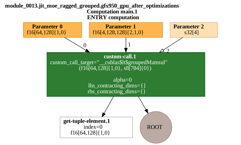
The measured attribution used fixed-capacity expert execution. The following optimized-HLO fixture uses tokens[64,128] and four expert matrices to show the signature of a sparse ragged path. Its ragged_dot_general lowers to the compatibility target __cublas$lt$groupedMatmul, which reaches the BLASLt implementation on ROCm.

Literal gfx950 optimized HLO rendered with Graphviz. The custom-call target is the bridge between the JAX ragged-dot name and the grouped GEMM kernel sought in rocprofv3. This is compiler evidence, not a performance measurement.

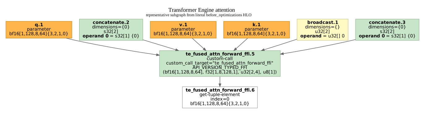
The attention path has the same pattern. In the retained Transformer Engine fixture, Q, K, V, and metadata enter custom_call_target="te_fused_attn_forward_ffi". The call identifies the framework-to-runtime handoff; the rocprofv3 trace identifies the kernels that implemented it.

Real pre-optimization HLO fixture for the Transformer Engine attention route. Use its custom-call and source names for attribution, then use the ROCm trace for the actual backend kernels and durations.

Verifying time attribution

Internal reconciliation proves that the ledger counts each row once; it does not prove that the semantic attribution is plausible. An external comparison should therefore match denominators before comparing ratios. Absolute durations are not useful here because accelerator, framework, sequence length, batch size, training method, and sharding all differ.

A close peer-reviewed comparison is Xia et al., “Understanding the Performance and Estimating the Cost of LLM Fine-Tuning”, published at IEEE IISWC 2024. The study profiles Mixtral 8x7B QLoRA on one NVIDIA A40. Although it uses the smaller Mixtral, it preserves the relevant architecture: eight SwiGLU experts, top-2 sparse routing, attention followed by an MoE block, and gradient checkpointing. Its Figure 5 divides combined forward and backward model time among normalization, attention, and MoE; Figure 6 then divides the MoE work among routing, top-k selection, dequantization, and the expert W1/W2/W3 matrix multiplications.

The paper reports that MoE consumes 85% of model-layer time on average across its experiments. For the closer sparse-Mixtral subset, the authors’ released Figure 5 measurements give MoE shares of 87.6% to 92.0%, with an unweighted mean of 90.3%. These ratios are computed from the released numbers, not estimated from the plotted bar heights.

To construct the matching ratio for this capture, exclude communication, optimizer/loss, and unattributed work because the IISWC layer breakdown is single-GPU model execution. Include rematerialized MoE work because that study includes checkpoint replay within backward time. Local forward MoE time is the router, dispatch, Expert MLP, and combine sum:

\[T_{\mathrm{MoE}} =1{,}857.4+6{,}065.2+2{,}197.2 =10{,}119.8\ \mathrm{ms},\]

and the matched model-compute denominator is

\[T_{\mathrm{model}} =2{,}322.8+7{,}287.9+2{,}210.5 =11{,}821.2\ \mathrm{ms}.\]

The resulting MoE share is 85.6%. It is 2.0 percentage points below the lowest sparse-Mixtral bar and 4.7 points below their sparse-Mixtral mean, but it has the same dominant proportion. The difference has plausible workload causes: the external run uses sequence length 128 and QLoRA targeted at the MoE modules, whereas this run uses sequence length 4,096 and computes full attention and expert weight gradients.

Matched check	IISWC Mixtral 8x7B	This Mixtral 8x22B capture	Assessment
MoE share of local model time	87.6–92.0% for sparse runs	85.6%	Same dominant fraction; modestly lower here
Backward / forward time	1.71–1.93× for sparse runs	3.14× excluding replay; 4.09× including replay	Same ordering; larger under full-weight training
Largest work inside MoE	W1/W2/W3 matrix multiplications	Expert MLP is 83.0% of local forward MoE time	Same kernel-level concentration

The phase range in the table comes from the study’s released Figure 4 measurements. The backward ratio is not expected to match: the paper explicitly notes that QLoRA computes gradients for only a small parameter subset, while this pretraining step differentiates all model weights.

There is also a model-identical, though not peer-reviewed, systems comparison. NVIDIA’s “MoE Parallel Folding” preprint profiles BF16 Mixtral 8x22B training on H100 GPUs. Its Figure 5 splits MoE-layer latency into router, FFN, permutation, AllToAll, and AllGather/ReduceScatter time over several EP/ETP mappings. FFN is the largest local component in every standard Mixtral 8x22B bar, while the paper finds that less favorable mappings increase the communication fraction and that crossing the eight-GPU NVLink domain sharply increases latency.

That result supports the two main features of this attribution: expert GEMMs dominate local model work, and communication can become the system bottleneck. It does not provide a numerical check for the 54.6% communication share above. The NVIDIA figure covers only the MoE layer on H100, with fixed attention TP, varying EP/ETP mappings, and token dropping; this capture covers the complete step on eight MI355X GPUs with FSDP=4/EP=2 and includes FSDP parameter and gradient collectives. The external evidence therefore validates the proportions and bottleneck ordering, not the absolute milliseconds or the communication percentage.

Captured end-to-end result

An earlier, independent timing run used the same model, batch, precision, and v26.6 FSDP=4/EP=2 fixed-capacity strategy. It remains the unprofiled timing anchor:

Field	Captured or derived value
Hardware	one node, 8× MI355X
Workload	synthetic, sequence 4,096, global batch 64
Recorded step samples	1
Step time [measured]	20.599 s
Instrumented XPlane step [measured]	20.605 s
Tokens/s/device [derived from measured step]	1,590.7
Useful TFLOP/s/device [derived from measured step and model ledger]	385.3
BF16 MFU [derived]	15.31%

The MFU uses the 2.5166 PFLOP/s dense-BF16 peak from Chapter 1:

\[\mathrm{MFU}=\frac{385.3}{2516.6}=0.1531.\]

The instrumented step differs from the independent timing sample by 0.03%. That agreement supports using the XPlane to explain the original result, but one independent timing sample is still insufficient for a variance estimate.

Component roofline worksheet

MaxText’s useful training-FLOP convention counts forward matrix work and twice that work for backward. The table applies that factor of three to the Q/K/V/O projections, causal attention, router, selected expert matrices, and language model head. It does not count the optimizer.

Component	Formula basis	Useful PFLOPs/update [analytical]	Share
Attention projections	Q, K, V, O across 56 layers	7.758	12.22%
Causal attention core	QK and probability-V products	2.217	3.49%
Router	$D\times8$ gate in 56 layers	0.004	0.007%
Two selected experts	two SwiGLU experts, three matrices each	53.199	83.78%
Output vocabulary head	$D\times32{,}768$	0.317	0.50%
Total	242.212 GFLOPs/token × 262,144 tokens	63.495	100%

This table estimates useful algorithmic work rather than executed hardware work. It excludes norms, sorting, token movement, collectives, optimizer arithmetic, padding, dropped assignments, and rematerialized repeats. Those operations remain in the time and byte ledgers.

The final objective is a component ledger that links model structure, compiler output, runtime behavior, and hardware measurements.

Worksheet field	XPlane/HLO source	ROCm source
Scope and HLO IDs	optimized HLO name stack, custom-call target	correlated kernel prefix
Local shapes and dtype	HLO operands/results and shardings	grid/workgroup and kernel metadata
Occurrences	Kernel Stats and loop body	dispatch IDs in one complete step
Device time	union of GPU events on critical device	normal trace start/end timestamps
Useful FLOPs	analytical model ledger	carried unchanged
Executed FLOPs	optimized shapes, padding, remat, backend contract	validated instruction/counter metrics
HBM bytes	XLA estimate, clearly labeled	counter-derived read/write bytes
Communication bytes	HLO collective shape and replica groups	RCCL payload/trace records
Arithmetic intensity	executed FLOPs / measured HBM bytes	derived from retained counters
Roofline efficiency	matching dtype peak and memory level	recomputed point and counter provenance

A complete performance investigation should retain enough information to reconstruct every attribution decision.

That means preserving the resolved configuration, optimized HLO, memory analysis, XSpace, runtime trace, counter methodology, and component ledger. With those artifacts, the reported roofline and attribution results remain reproducible long after the original run has been discarded.

Next: training in mixed precision.