Sharding and Parallelism
Chapter 5 of How to Scale Your Model on AMD (Chapter 4: Training in Mixed Precision | Chapter 6: Memory and Kernel Optimizations)
How JAX and Shardy turn global arrays into local MI355X work, how FSDP and expert parallelism use collectives, and how to choose a MaxText mesh.
A JAX program is written as if every tensor exists as a single global array. During compilation, that global program is transformed into one executable per device, each operating on local tensor shards and communicating with its peers when necessary.
Sharding therefore determines three key properties of the resulting system:
- which tensor dimensions are split;
- which named mesh axes perform each split; and
- which physical devices occupy the mesh coordinates.
FSDP, ZeRO, tensor parallelism, and expert parallelism are all recurring ways of choosing those mappings. They are often described as distinct training strategies, but from the compiler’s perspective they are all expressed through the same mechanism: array sharding and collective communication. On ROCm, those collectives use the RCCL runtime.
Sharding as a compiler transformation
Global arrays and device-local shards
Consider a global array
\[A[d_0,d_1,\ldots,d_{n-1}]\]and a PartitionSpec that maps array dimension $i$ to a set of mesh axes
$S_i$. If the axes in $S_i$ have total size
then an evenly partitioned device stores
\[A_{\mathrm{local}} \left[ \frac{d_0}{q_0}, \frac{d_1}{q_1}, \ldots, \frac{d_{n-1}}{q_{n-1}} \right].\]For an element size of $s$ bytes, the local payload is
\[M_{\mathrm{local}} =s\prod_i\frac{d_i}{q_i}.\]In the ideal case, every sharded dimension divides evenly across the participating mesh axes. When that is not possible, the compiler may need to introduce padding or choose a different partitioning strategy. A mesh axis also cannot partition two different dimensions of the same array at once.
One useful consequence of JAX’s global-array model is that the logical shape
never changes from the user’s perspective. The local buffers are visible
through addressable_shards. An array can report shape (1024, 512) even
though each of eight devices stores only (128, 512). The
JAX distributed-array guide
defines this global view and the relationship among Mesh,
PartitionSpec, and NamedSharding.
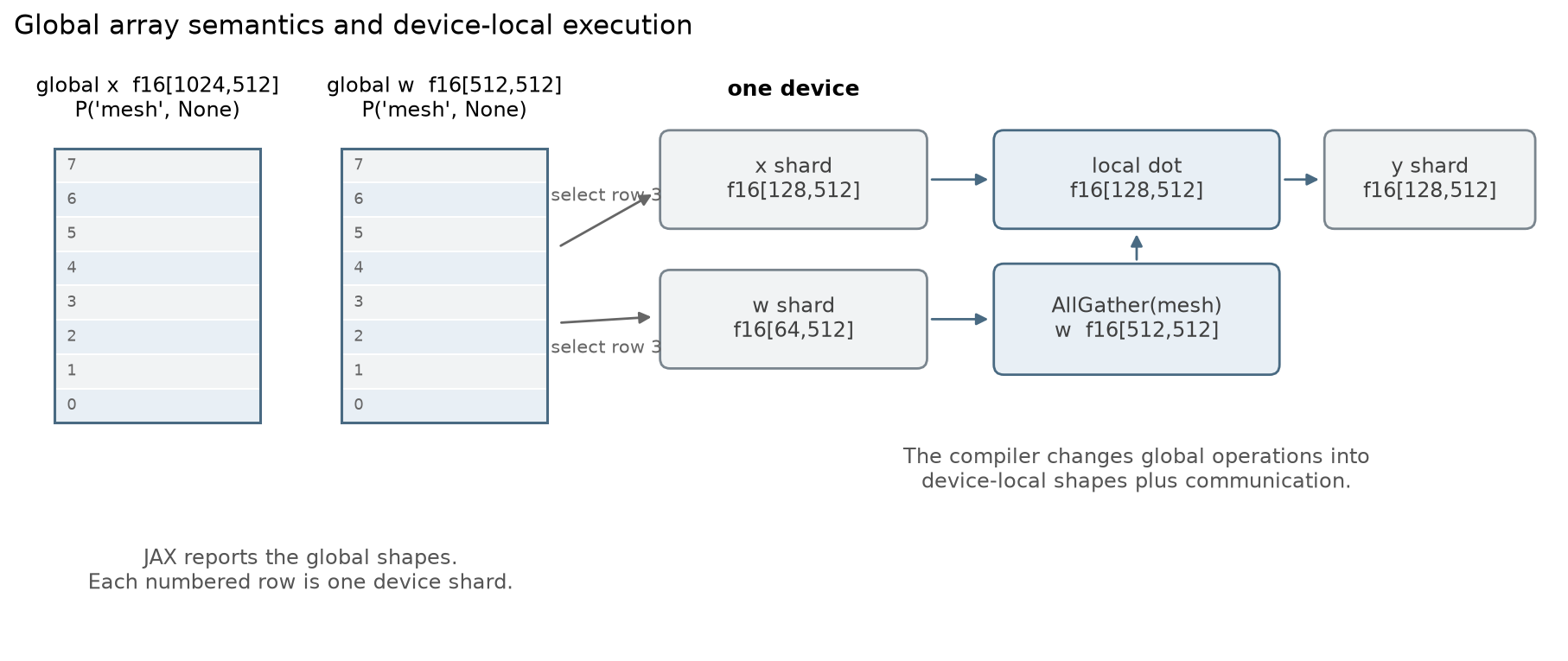
The figure also highlights a common misconception about accelerator memory. Eight MI355X OAMs provide eight separate 288 GB HBM allocations. A sharded array places a slice in each allocation; a replicated array places a full copy in each. The 2.304 TB physical total is not one allocator.
Shardy propagation, resharding, and partitioning
Shardy is the mechanism OpenXLA uses to reason about shardings throughout the compilation process. It carries mesh and layout information through the compiler and determines how global operations become local computations and collectives. Its propagation pass follows operation sharding rules in both directions until it reaches a fixed point. For a matmul written as
\[(i,k),(k,j)\rightarrow(i,j),\]the rule relates matching batch, contracting, and non-contracting factors across the two operands and result.
Propagation alone is not enough. Two operations may still require incompatible layouts, forcing the compiler to change how data is distributed. The current Shardy export pipeline makes the remaining work explicit:
sdy-insert-explicit-reshardsinserts a reshard where an operation cannot consume the propagated operand layouts directly.sdy-reshard-to-collectivesconverts those reshards to collective operations.- divisibility handling and global-to-local conversion produce device-local shapes.
- in current mixed pipelines, Shardy can partition selected instructions and
wrap their local code in
sdy.manual_computation; downstream XLA SPMD partitioning handles the remaining global instructions.
The implementation details continue to evolve as Shardy replaces older partitioning paths, but the observable behavior remains the same: sharding annotations enter the compiler, while local tensor shapes and communication operations emerge from the partitioned program.
An FSDP policy asks for parameter, gradient, and optimizer-state layouts along an FSDP axis. An expert-parallel policy maps the expert dimension and routed activations to an expert axis. Shardy implements the consequences of those array layouts; it does not decide that a model should use FSDP or EP.
The cost of the inserted collectives
The most important consequence of sharding is that communication becomes part of the training step.
Whenever the partitioned program requires data that is distributed across devices, the compiler inserts collectives such as AllGather, ReduceScatter, AllReduce, and AllToAll. Their costs often determine whether a particular sharding strategy scales efficiently.
Let $X$ be the number of participating devices, $B$ the size in bytes of the completed AllGather buffer, and $W$ the achieved one-direction bandwidth of the link used by one ring hop. Each device begins with $B/X$ bytes. A ring sends that chunk once per round for $X-1$ rounds:
\[T_{\mathrm{AG,ring}} \geq \frac{B(X-1)}{XW}.\]

A ring ReduceScatter has the same transport term. It starts with a reducible $B$-byte buffer on each rank and leaves $B/X$ bytes on each:
\[T_{\mathrm{RS,ring}} \geq \frac{B(X-1)}{XW}.\]A ring AllReduce is a ReduceScatter followed by an AllGather:
\[T_{\mathrm{AR,ring}} \geq \frac{2B(X-1)}{XW}.\]For AllToAll, let each rank begin with a local payload of $L$ bytes, divided into $X$ destination blocks. Each rank sends $L(X-1)/X$ bytes remotely. With achieved aggregate egress bandwidth $W_X$,
\[T_{\mathrm{A2A}} \geq \frac{L(X-1)}{XW_X}.\]On the MI355X UBB, an $X$-GPU subgroup has $X-1$ direct peer links per GPU, each with a 76.8 GB/s directional line-rate ceiling. If an implementation uses all participating links concurrently, then
\[W_X\leq(X-1)(76.8\ \mathrm{GB/s}) \quad\Longrightarrow\quad T_{\mathrm{A2A}} \geq \frac{L}{X(76.8\ \mathrm{GB/s})}.\]This should be interpreted as a best-case lower bound rather than a runtime prediction. Real implementations must also pay launch overheads, synchronization costs, protocol overheads, and algorithm-specific inefficiencies. The relevant $W$ is achieved directional bandwidth for the message size, never AMD’s doubled bidirectional figure. The Scaling Book sharding chapter derives the same collectives from matrix layouts, while its GPU chapter develops the ring cost model.
Real HLO before and after partitioning
The easiest way to understand partitioning is to inspect the HLO before and after Shardy has transformed the program.
The explanatory fixtures below were compiled on eight GPUs with JAX 0.11.0 in the MaxText v26.6 ROCm environment using:
XLA_FLAGS="--xla_dump_hlo_as_text --xla_dump_hlo_as_dot ..." \
  python -m bench.hlo_feature_fixtures sharding fsdp
The retained capture includes the source text, DOT graph, command, and compiler options. Graphviz renders representative subgraphs from XLA’s DOT output. Operation names, shapes, and sharding values come directly from the dump. Redundant attribute wrappers and source tooltips are pruned, and dependency arrows may contract omitted tuple or copy nodes. These fixtures explain compilation and are not performance measurements.
Before partitioning, the compiler still sees a global computation. In the
FSDP-style fixture, x and w both have global shapes, and their
xla.sdy.sharding attributes split dimension 0 over the eight-device mesh.
xla.sdy.FuncResultSharding records the requested result layout. It is a
compiler marker, not an external runtime kernel.
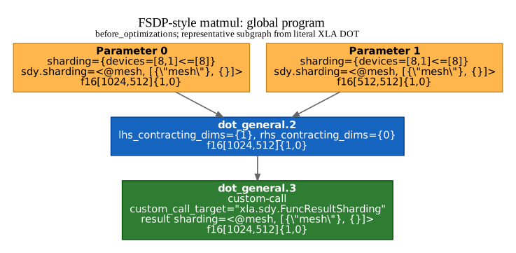
Representative subgraph from the literal pre-optimization graph; open the SVG to read the full annotations.
After partitioning, the same computation has become a device-local program.
The entry parameters now have local shapes: x is f16[128,512], w is
f16[64,512], and the generated all-gather reconstructs w as
f16[512,512] before the dot. The local output remains f16[128,512].
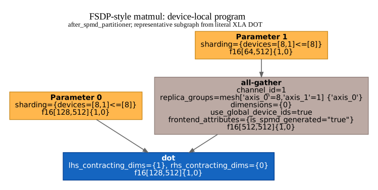
Representative subgraph from the literal post-partitioner graph.
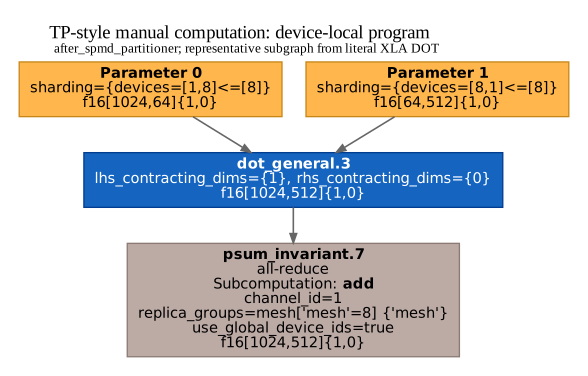
The tensor-parallel fixture uses jax.shard_map. It shards the contracting
dimension of both operands, computes a partial dot on each device, and calls
jax.lax.psum. Its global wrapper therefore already contains an explicit
all-reduce before downstream SPMD partitioning. The representative view
keeps the manual body’s dot and collective:
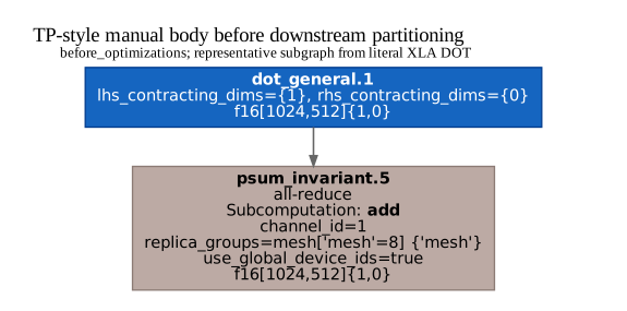
After partitioning, copies around the manual-computation boundary can be
removed from the instructional view. The local f16[1024,64] and
f16[64,512] operands produce a f16[1024,512] partial result, then the
eight-way all-reduce sums those partials:
The three matched fixtures make the role of layout precise:
| Fixture | Global layout | Device-local HLO | Collective in retained artifact |
|---|---|---|---|
| data parallel | x[1024,512] row-sharded; w[512,512] replicated |
x[128,512] @ w[512,512] |
none |
| FSDP style | x and w row-sharded |
AllGather(w[64,512]) → w[512,512]; local dot |
all-gather |
| TP style | contracting dimensions split | x[1024,64] @ w[64,512]; sum partial outputs |
all-reduce |
These artifacts contain no reduce-scatter, all-to-all, or
collective-permute, so the graphs do not claim otherwise. A complete
training-step backward pass commonly adds a gradient ReduceScatter for FSDP,
and an MoE dispatch commonly adds AllToAll. Those claims must be checked
against that step’s own post-partitioner HLO.
Parallelism strategies
The Scaling Book develops the underlying theory. For this chapter, the important question is simpler:
What object is being split, and what communication does that split introduce?
| Strategy | What is split | Typical communication | Main constraint |
|---|---|---|---|
| replicated data parallelism | batch only; full model on every rank | gradient AllReduce | full model state must fit one device |
| ZeRO-1 | batch and optimizer state | gradient reduction and updated-parameter exchange | parameters and gradients remain replicated |
| ZeRO-2 | batch, gradients, optimizer state | gradient ReduceScatter and updated-parameter AllGather | parameters remain replicated |
| FSDP / ZeRO-3 | batch, parameters, gradients, optimizer state | parameter AllGather and gradient ReduceScatter | gather buffers and communication must fit the schedule |
| tensor parallelism | hidden, head, or MLP dimensions | activation AllReduce or AllGather/ReduceScatter | local GEMMs must remain efficient |
| expert parallelism | expert dimension | routed-token AllToAll and combine | expert load balance and token payload |
The original ZeRO paper defines the stages by cumulative partitioning of optimizer state, gradients, and parameters. Libraries differ in scheduling details, so the HLO and profile remain authoritative for a specific program.
FSDP and ZeRO
Let a model have $P$ parameters, with $b_p$ bytes of parameter storage, $b_g$ bytes of gradient storage, and $b_o$ bytes of optimizer state per parameter. Fully replicated persistent state requires approximately
\[M_{\mathrm{replicated}}=P(b_p+b_g+b_o).\]Ideal $X$-way full sharding reduces that persistent term to
\[M_{\mathrm{FSDP,persistent}} \approx\frac{P(b_p+b_g+b_o)}{X}.\]The peak is higher because the current layer’s parameter buffer can be AllGathered, activations remain live, and the compiler and libraries allocate temporaries. FSDP therefore trades memory capacity for communication. Persistent replicated state becomes smaller, but transient gather buffers and collective operations become part of every training step.
The throughput tradeoff follows from the same decision. For
\[X_{\mathrm{local}}[B/X,D]\, W_{\mathrm{local}}[D/X,F],\]the forward pass gathers $W[D,F]$ before the dot. The backward pass reduces and scatters the corresponding gradient. Increasing $X$ lowers persistent state per rank, but it also lowers token rows per rank and leaves less compute with which to overlap each layer’s communication. Pure data parallelism avoids the forward weight gather but keeps the full state replicated.
Dense models have no expert axis to exploit. Their capacity plan usually uses some combination of FSDP, tensor parallelism, sequence/context parallelism, and pipeline parallelism. Which combination wins depends on local GEMM shapes, batch size, memory, topology, and exposed collective time.
Expert parallelism
Unlike dense models, MoE architectures already contain a natural dimension that can be distributed: the experts themselves. For expert weights
\[W_{\mathrm{expert}}[E,D,H],\]a size-$Z$ EP axis can store
\[W_{\mathrm{local}}[E/Z,D,H].\]The router selects $k$ experts for each token. If the selected experts live on other ranks, dispatch moves token rows to their owners and combine returns the expert outputs. These are usually AllToAll-shaped exchanges. Expert parallelism reduces local expert storage and divides expert computation across devices, but it introduces a new requirement: tokens must be moved to the devices that own their selected experts.
A dense model has $E=1$, so an EP axis cannot split its MLP weights. An MoE still needs other axes for attention, embeddings, optimizer state, or further splitting inside each expert. FSDP and EP can therefore be orthogonal:
\[W[E_{\mathrm{ep}},D_{\mathrm{fsdp}},H].\]The local shape is
\[\left[\frac{E}{Z},\frac{D}{X},H\right]\]on an (fsdp=X, ep=Z) mesh. This two-axis layout is the basis of the Mixtral
case study.
DeepSeek-V3 high-EP mesh
DeepSeek-V3 provides a useful example of these ideas applied at frontier scale. Its 671B-parameter MoE has 256 routed experts and selects 8 per token. Training used:
- 2,048 H800 GPUs;
- 16-way pipeline parallelism;
- 64-way expert parallelism spanning eight nodes;
- ZeRO-1 data parallelism; and
- no tensor parallelism in the reported training configuration.
The 16-way PP and 64-way EP axes consume $16\times64=1{,}024$ devices per model-parallel replica. With 2,048 devices, the remaining data-parallel degree is two. The report also describes custom cross-node AllToAll kernels and the DualPipe schedule used to overlap communication with forward and backward compute.
DeepSeek-V3 should not be treated as a universal mesh template. Instead, it demonstrates that sufficiently large MoE models can justify dedicating a substantial fraction of the system to an expert-parallel axis.
Implementing sharding in JAX
Mesh, NamedSharding, and PartitionSpec
JAX exposes sharding through three closely related concepts.
A Mesh assigns names to dimensions of an array of devices. A
PartitionSpec maps tensor dimensions to those names. A NamedSharding pairs
the two. The
JAX sharding API
defines all three.
The following JAX 0.11 example creates a two-by-four logical mesh on eight devices. The activation batch is split across both axes. The weight’s contracting dimension is split only over FSDP and is replicated across EP:
from functools import partial

import jax
import jax.numpy as jnp
import numpy as np
from jax.sharding import Mesh, NamedSharding, PartitionSpec as P

devices = np.asarray(jax.devices()).reshape(2, 4)
mesh = Mesh(devices, ("fsdp", "ep"))

x_s = NamedSharding(mesh, P(("fsdp", "ep"), None))
w_s = NamedSharding(mesh, P("fsdp", None))
y_s = NamedSharding(mesh, P(("fsdp", "ep"), None))

x = jax.device_put(jnp.ones((1024, 512), jnp.bfloat16), x_s)
w = jax.device_put(jnp.ones((512, 512), jnp.bfloat16), w_s)

@partial(jax.jit, in_shardings=(x_s, w_s), out_shardings=y_s)
def linear(x, w):
  x = jax.lax.with_sharding_constraint(x, x_s)
  return x @ w

y = linear(x, w)
print(x.shape, x.addressable_shards[0].data.shape)
# (1024, 512), (128, 512) on this one-process eight-device mesh
Although the program operates on global shapes, each device only stores the
shard implied by its coordinates in the mesh. In this example, each device
stores x[128,512] and w[256,512], with each FSDP weight shard replicated at
the four EP coordinates. The dot needs the full contracting dimension, so the
automatic partitioning path can insert an FSDP AllGather.
P(None, None) is replicated with respect to every mesh axis. A tuple such as
P(("fsdp", "ep"), None) applies the product of both named axes to one tensor
dimension. Unused mesh axes imply replication, which consumes memory even
though the global shape is unchanged.
Constraints and compilation boundaries
jax.jit accepts shardings or matching pytrees through in_shardings and
out_shardings. Inputs must be compatible with the declared layouts.
out_shardings constrains the returned layout. The
current jax.jit reference
documents those boundary checks.
jax.lax.with_sharding_constraint constrains an intermediate. Under automatic
mesh axes it gives Shardy another layout decision from which to propagate.
Sharding constraints are useful because they remove ambiguity, but they can
also be overused. Too few constraints may leave an important layout decision
unspecified, while too many can force unnecessary resharding between adjacent
operations. Inspect post-partitioner HLO after changing one.
JAX 0.11 also supports explicit mesh-axis types. In explicit mode, sharding is
part of the trace-time array type and operation rules propagate it in JAX.
Automatic mode leaves more intermediate decisions to Shardy. The
JAX explicit-sharding guide
and the
Scaling Book JAX chapter
compare jax.jit automatic and explicit axes with jax.shard_map.
jax.shard_map changes the programming view. Its function body sees local
arrays, and the programmer writes collectives such as jax.lax.psum
explicitly. The TP HLO fixture above uses that route. It is useful when the
automatic global program does not express the required algorithm clearly.
Orthogonal axes and physical placement
Mesh axes are independent dimensions of the logical device grid. Their sizes multiply together to determine the number of required devices. A mesh with
fsdp: 8
expert: 8
contains
\[8\times8=64\]device coordinates. It cannot place both independent size-eight axes on the
same eight devices. On one eight-GPU node, the four two-axis choices with
product eight are (1,8), (2,4), (4,2), and (8,1).
Mesh shape does not describe the network. reshape(2, 4) assigns logical
coordinates according to the order of jax.devices(). It does not assert that
rows share a NIC rail, that columns stay inside one host, or that adjacent
coordinates have a faster link. On a single MI355X UBB, all eight GPUs have
one-hop xGMI links to one another, which makes logical order less restrictive.
Across nodes, construct the device array from the actual host, GPU, and NIC
mapping.
MaxText from flags to shardings
The pinned MaxText source path
Conceptually, MaxText performs the following transformation:
YAML → Mesh → logical axes → NamedSharding → jax.jit → Shardy →
local HLO.
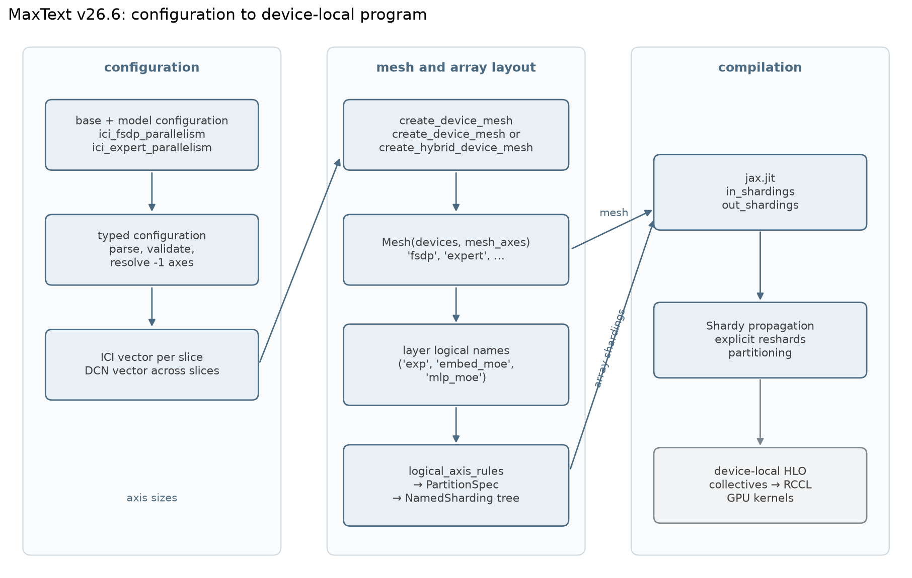
The source references below trace that transformation through the MaxText
release/v26.6 tree at commit
b47d74bf:
base.ymldefinesmesh_axes, logical-axis rules, and ICI/DCN axis sizes.types.pygives these fields typed defaults.create_device_meshorders the ICI sizes according tomesh_axes, resolves one-1dimension, and calls JAX’screate_device_meshorcreate_hybrid_device_mesh.get_mesh_from_configwraps that device array inMeshand selects automatic or explicit axis types fromshard_mode.- Layers attach logical names to parameters and activations. Mixtral creates
its routed MoE in
mixtral.py. The expert matrices use logical axes such asexp,embed_moe, andmlp_moeinmoe.py. - MaxText converts the resulting logical annotation tree to concrete mesh
shardings in
get_abstract_state. - The state and data sharding pytrees become
jax.jitinput and output shardings injit_train_step. MaxText then setsjax_use_shardy_partitionerfrom theshardyfield intrain.py.
The JAX Shardy migration guide
states that Shardy became JAX’s only partitioner after March 2026. In the JAX
0.11 environment used here, keep shardy: true; the MaxText field remains a
compatibility surface, not a choice between two supported partitioners.
For the two-axis Mixtral meshes in this chapter, the relevant configuration is:
hardware: gpu
num_slices: 1
shard_mode: auto
shardy: true

ici_fsdp_parallelism: 2
ici_expert_parallelism: 4
dcn_fsdp_parallelism: 1
dcn_expert_parallelism: 1
The default rules include:
['activation_batch_moe',
 ['data', 'fsdp', 'fsdp_transpose', 'expert']]
['exp', 'expert']
['embed_moe', ['fsdp', 'fsdp_transpose', 'context']]
['mlp_moe',
 ['fsdp_transpose', 'tensor', 'tensor_sequence', 'autoregressive']]
With only fsdp and expert larger than one, an expert up-projection annotated
as ("exp", "embed_moe", "mlp_moe") resolves to the effective physical spec
P("expert", "fsdp", None)
for its [experts, input, output] dimensions. MaxText can also remove
expert from the dispatched activation’s batch dimension so that the expert
dimension remains on EP and the compiler emits the intended token exchange.
The behavior is named by
moe_dispatch_no_expert_sharding
and implemented in
_maybe_shard_moe_dispatch.
The YAML numbers are therefore only the first step. The logical names on each
parameter and activation, the rule table, and any route-specific constraint
determine the emitted NamedSharding.
ICI and DCN on ROCm
MaxText uses ICI for the mesh shape within one slice and DCN for the
shape across slices. These names originated in TPU-oriented configuration.
They are logical hierarchy names when hardware: gpu; they do not identify a
ROCm transport by themselves.
For this one-node case, num_slices: 1, all DCN dimensions are one, and the ICI
shape contains the eight visible GPUs. Given the device order used here, that
mesh remains within the UBB’s xGMI scale-up domain.
When num_slices > 1, MaxText’s hybrid mesh constructor combines ICI and DCN
vectors. On an MI355X cluster, the operator still has to establish:
- which JAX processes and devices belong to each host;
- how local GPU indices map to NIC rails;
- which collective backend and RDMA path are active; and
- whether each named axis remains local or crosses the scale-out network.
Setting dcn_expert_parallelism: 8 does not create an eight-way 400 Gb/s
fabric or guarantee rail alignment. Treat it as a requested logical placement,
then verify the device array and profile the resulting RCCL traffic.
Case study: Mixtral 8x22B
Mixtral 8x22B has about 141B total
parameters and 39B active parameters per token. The MaxText v26.6
mixtral-8x22b.yml
uses 56 layers, model width 6,144, expert MLP width 16,384, eight experts, and
top-2 routing.
The local experiment fixes:
- one node with eight MI355X devices;
- BF16 parameters and compute, with FP32 gradients;
- sequence length 4,096;
- four sequences per device per microstep;
- two gradient-accumulation microsteps; and
- a global update of 64 sequences, or 262,144 token positions.
Only the FSDP and EP degrees change in the mesh study.
Four one-node mesh cells
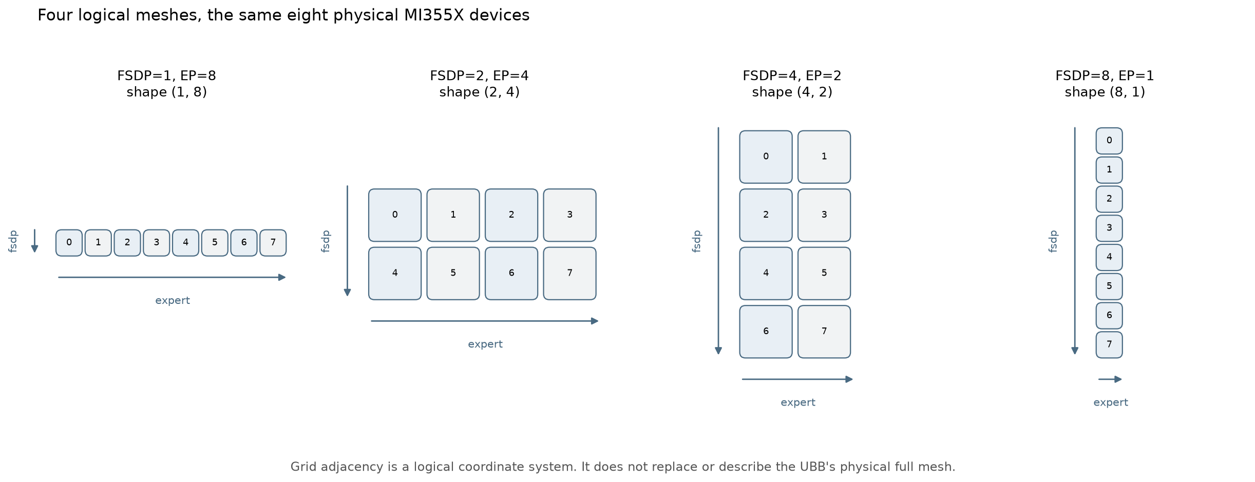
| FSDP | EP | Batch placement | Expert-weight placement | Dominant communication family to inspect |
|---|---|---|---|---|
| 1 | 8 | token batch split eight ways | one expert per rank | token dispatch/combine AllToAll |
| 2 | 4 | token batch split eight ways | two experts, each split two ways | AllToAll plus parameter AllGather/gradient ReduceScatter |
| 4 | 2 | token batch split eight ways | four experts, each split four ways | smaller EP group, larger FSDP group |
| 8 | 1 | token batch split eight ways | all experts, each split eight ways | parameter AllGather/gradient ReduceScatter |
The final column is a hypothesis derived from the layouts. Collective count, message size, combining, rematerialized gathers, and overlap come from HLO and the runtime profile.
Parameter memory
The published rounded parameter count gives a BF16 parameter payload of
\[M_{\mathrm{params}}=(141\times10^9)(2\ \mathrm{bytes}) =282\ \mathrm{GB}.\]If every parameter is evenly sharded across the product $X_{\mathrm{fsdp}}X_{\mathrm{ep}}=8$, the ideal persistent parameter payload is
\[M_{\mathrm{params,local}} =\frac{282}{8} =35.25\ \mathrm{GB/device}.\]This is a parameter-only lower bound based on a rounded model count. Small or indivisible leaves can be replicated, and training also needs gradients, optimizer state, activations, collective buffers, and compiler workspaces.
The dominant expert matrices give a more exact layout check. Each layer has two up-projection matrices and one down-projection matrix:
\[\begin{aligned} W_{i0},W_{i1}&:[8,6144,16384],\\ W_o&:[8,16384,6144]. \end{aligned}\]Each contains 805,306,368 elements, or 1,610,612,736 BF16 bytes (1.611 GB, 1.5 GiB). All four mesh cells store one eighth of each matrix per rank:
\[\frac{1{,}610{,}612{,}736}{8} =201{,}326{,}592\ \mathrm{bytes}.\]Across three expert matrices and 56 layers, these expert weights alone account for 270.583 GB globally and 33.823 GB per device under ideal eight-way sharding. That agreement with the 35.25 GB whole-model estimate is a useful configuration check.
Communication predictions
For one expert up- or down-projection, the effective layout is
\[[8_{\mathrm{ep}},6144_{\mathrm{fsdp}},16384].\]An FSDP gather reconstructs the input dimension for the local expert subset. In a ring, every round sends the same 201.327 MB local shard. The table gives transport bytes per rank for one matrix use:
| FSDP / EP | Persistent local shape | Shape after FSDP gather | Ring AllGather bytes sent per rank |
|---|---|---|---|
| 1 / 8 | [1,6144,16384] |
no gather | 0 MB |
| 2 / 4 | [2,3072,16384] |
[2,6144,16384] |
201.327 MB |
| 4 / 2 | [4,1536,16384] |
[4,6144,16384] |
603.980 MB |
| 8 / 1 | [8,768,16384] |
[8,6144,16384] |
1,409.286 MB |
At the 76.8 GB/s per-peer xGMI line-rate ceiling, the ring serialization terms for the last three rows are 2.62 ms, 7.86 ms, and 18.35 ms per matrix. A ReduceScatter of the matching BF16 gradient has the same ideal ring byte term. Actual gradients are configured as FP32 in this experiment, so a materialized FP32 gradient payload would double these byte counts unless the implementation casts or accumulates differently.
The EP side begins with token rows. Across one optimizer update, each rank owns
\[\frac{262{,}144}{8}=32{,}768\]token positions before expert dispatch. With top-2 routing, BF16 width 6,144, and perfectly packed rows, the per-rank routed payload for one layer is
\[L=(32{,}768)(2)(6{,}144)(2\ \mathrm{bytes}) =805{,}306{,}368\ \mathrm{bytes}.\]The remote portion of one dispatch or combine exchange is:
| FSDP / EP | EP ranks | Packed payload sent off-rank per device and layer |
|---|---|---|
| 1 / 8 | 8 | 704.643 MB |
| 2 / 4 | 4 | 603.980 MB |
| 4 / 2 | 2 | 402.653 MB |
| 8 / 1 | 1 | 0 MB |
These values count useful routed rows and the two selected experts. They exclude indices, alignment, capacity padding, load imbalance, and duplicate internal representations. The fixed-capacity one-hot path can therefore move a different buffer. Gradient accumulation also splits the update payload across two microsteps.
The direct-link serialization bound illustrates why bytes alone are insufficient. If every EP peer link is active concurrently, the EP=8 row has an ideal 1.31 ms transport term per exchange, while EP=2 has 5.24 ms. EP=8 sends more total remote bytes but has seven direct links and smaller per-destination blocks. RCCL efficiency, latency, and the actual dispatch layout determine whether that physical advantage is realized.
Increasing FSDP shifts this example toward parameter AllGather and gradient ReduceScatter. Increasing EP shifts it toward token AllToAll. The model has three expert matrices and 56 layers, with dispatch and combine in forward and backward computation. Compiler reuse, rematerialization, collective combining, and overlap decide how many predicted transfers reach the critical path.
Successful measurements
The supplied Mixtral result summary contains one complete v26.6 mesh cell under the fixed-capacity configuration:
| Mesh | Step time | TFLOP/s/device | Tokens/s/device |
|---|---|---|---|
| FSDP=4, EP=2 | 20.599 s | 385.3 | 1,590.7 |
This measurement demonstrates that the configuration successfully executed, but it is insufficient for comparing mesh choices or estimating run-to-run variability.
A separate controlled sweep provides supporting systems evidence. It uses
deepseek2-16b, not Mixtral, on one eight-MI355X node. Every row used the same
model and workload; train-step statistics cover post-warmup steps 10–29.
The RCCL columns come from separate rocprofv3 jobs over steps 10–12.
deepseek2-16b mesh |
Mean step | TFLOP/s/device | Tokens/s/device | RCCL active | RCCL overlapped | Exposed RCCL |
|---|---|---|---|---|---|---|
| FSDP=8, EP=1 | 0.9478 s | 283.6 | 17,286.2 | 235.2 ms | 17.5% | 194.1 ms |
| FSDP=4, EP=2 | 1.6856 s | 159.5 | 9,719.9 | 1,321.0 ms | 39.6% | 798.1 ms |
| FSDP=2, EP=4 | 1.4215 s | 189.1 | 11,526.6 | 890.1 ms | 42.2% | 514.4 ms |
| FSDP=1, EP=8 | 0.8591 s | 312.9 | 19,071.9 | 216.0 ms | 79.3% | 44.7 ms |
The result is not monotonic in FSDP or EP degree. In this sweep, the EP=8 endpoint has the shortest mean step and least exposed RCCL, while both mixed cells expose much more communication. The FSDP=8 endpoint is also faster than the mixed cells despite its low RCCL overlap percentage. Mesh labels alone do not explain the result; message layout, local kernels, and scheduling changed together.
A repeatable selection procedure
The workflow used throughout this chapter can be summarized as a simple rule:
Use analysis to narrow the search space, then use profiling to choose among the remaining candidates.
- Build the
Meshfrom an explicit device order and print its coordinates. - Print MaxText’s resolved parameter and input
NamedShardingtrees. Confirm local shapes and persistent bytes before compiling a full step. - Dump
before_optimizationsandafter_spmd_partitionerHLO for each mesh. Count collective operations by replica group, dtype, shape, and source scope. A count without bytes is not useful. - Run synchronized post-warmup timing with the model, batch, precision, rematerialization, and compiler flags held fixed.
- Trace the same steady-state steps with
rocprofv3. Measure RCCL active time, overlap with other GPU work, and exposed RCCL on the step’s critical rank. - Inspect local GEMM shapes. A mesh that reduces communication can still lose throughput if it leaves too few token rows or awkward expert matrices for the selected kernels.
This procedure separates a capacity result, a compiler result, and a runtime result. All three are needed before choosing the production mesh.
Extending the mesh across nodes
Chapter 1 established the available directional ceilings:
| Path | Directional line-rate ceiling | Scope |
|---|---|---|
| xGMI peer link | 76.8 GB/s | one direct peer inside the eight-GPU UBB |
| all seven xGMI links | 537.6 GB/s aggregate egress | one GPU communicating with seven peers |
| PCIe Gen 5 x16 | 64 GB/s | one OAM’s host/I/O path |
| 400 Gb/s reference NIC | 50 GB/s | one scale-out link before protocol overhead |
The first eight devices form a one-hop full mesh. A ninth device crosses the scale-out boundary. For a ring collective, placement changes the $W$ in
\[T_{\mathrm{AG/RS,ring}} \geq\frac{B(X-1)}{XW}.\]An all-local ring can use an xGMI peer edge whose directional ceiling is 76.8 GB/s. A ring that crosses nodes contains a slower path bounded by the deployed NIC, PCIe, switch fabric, routing, and protocol. For the Chapter 1 reference design, one 400 Gb/s NIC has a 50 GB/s line rate and the PCIe path has a 64 GB/s line rate, so that rail is bounded above by
\[W_{\mathrm{scale\ out}} \leq\min(64,50)\ \mathrm{GB/s} =50\ \mathrm{GB/s}\]before overhead. This is a per-rail ceiling, not a claim about an installed cluster’s aggregate bandwidth.
A hierarchical collective has work at both tiers. If its local phase has ideal time $T_{\mathrm{up}}$ and its network phase has ideal time $T_{\mathrm{out}}$, then perfect overlap cannot beat
\[T_{\mathrm{hierarchical}}\geq \max(T_{\mathrm{up}},T_{\mathrm{out}}),\]while a serialized implementation pays their sum. The buffer size at each tier depends on whether the implementation gathers locally, reduces locally, or stripes data across NIC rails first. Derive those tier-specific bytes from the post-partitioner shapes and RCCL algorithm rather than inserting the global tensor size into both terms.
AllToAll placement is especially sensitive to rails. In a rail-optimized
design, equal local GPU indices on different hosts can share a low-hop path.
An EP axis whose coordinates ignore that mapping can send traffic through a
spine or add a local xGMI hop before network egress. A JAX mesh name such as
expert carries no rail information.
For a larger run, keep high-volume, latency-sensitive axes inside the UBB when the model and memory allow it. Place an axis across nodes only after comparing its post-partitioner bytes with measured scale-out bandwidth and overlap. Chapter 1 intentionally gives no subscription ratio or switch topology for an unspecified deployment, so this chapter does not assign one.
References
- JAX distributed arrays and automatic parallelization: global arrays, meshes, automatic and explicit sharding.
- JAX sharding API:
Mesh,NamedSharding, andPartitionSpec. - OpenXLA Shardy, propagation, and export passes: propagation, explicit reshards, collectives, and global-to-local conversion.
- ROCm RCCL API: AllReduce, AllGather, ReduceScatter, and AllToAll semantics.
- JAX Scaling Book: sharded matrices, training parallelism, and JAX programming: generic derivations and programming models.
- DeepSeek-V3 Technical Report: 64-way EP, 16-way PP, ZeRO-1, and communication overlap.
- Mistral AI: Mixtral 8x22B: total and active parameter counts.
- ROCm MaxText v26.6 at
b47d74bf: the configuration, mesh, logical-axis, and JIT source traced above.
At this point the global training problem has been transformed into a collection of device-local computations. The chosen mesh determines the activation shapes, matrix sizes, and communication patterns seen by each MI355X.
The next chapter focuses on optimizing those local computations through rematerialization, attention kernels, and MoE execution strategies.